本記事は、「ライブラリーを使わずにPythonでニューラルネットワークを構築してみる - Qiita 」を
会社の先輩がChainerでやってみた記事(chainerでニューラルネットワーク構築 - Qiita)を
さらにKerasでやってみたものです(社内のLT向け資料です)
※注意 本記事は Keras 1.x 時代に書かれたものです。2.xでは未検証のため動作しない可能性があります。
全ソースと実行結果(Jupyter Notebook)
ソースと実行結果は以下のGistにあげています。
Kerasでニューラルネットワーク構築
実装と解説
データ作成
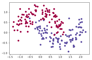
入力データを作成します。ここは全く同じ実装です。
import numpy as np
import sklearn.datasets
import matplotlib
import matplotlib.pyplot as plt

np.random.seed(0)
X,y=sklearn.datasets.make_moons(200,noise=0.20)
plt.scatter(X[:,0], X[:,1], s=40, c=y, cmap=plt.cm.Spectral)
モデル作成
Kerasでモデルを作成します。
import keras
from keras.models import Sequential
from keras.layers import Dense, Activation

model = Sequential()
model.add(Dense(output_dim=6, input_dim=2))
model.add(Activation('tanh'))
model.add(Dense(output_dim=2))
model.compile(optimizer='Adam', loss='mse')
Chainerのものを移植したのでだいたい同じです。
(ただし、損失関数に関してはChainerでは Classifier に隠蔽されてるらしいですが、何が使われてるんでしょう?)
=> [追記] 以下の記事では、ChainerのClassifierでは softmax_cross_entropy が使われているとのことでした。
Chainer1.5の変更点についてのメモ - studylog/北の雲
| 種別 | 設定値 |
|---|---|
| インプット層 | 2 |
| 隠れ層 | 6 |
| 活性化関数 | tanh |
| アウトプット層 | 2 |
| オプティマイザ(最適化アルゴリズム) | Adam |
| 目的関数(損失関数) | 平均二乗誤差 (Mean Squared Error) |
Sequentialモデルのガイド - Keras Documentation
活性化関数 - Keras Documentation
最適化 - Keras Documentation
目的関数 - Keras Documentation
(epochがChainerでは20000となっていたのを移植時にまちがえて2000にしてしまっていて、隠れ層がChainerと同じ3だといまいちな結果でした。だた隠れ層を6にしたところ2000でもわりといい結果が得られました)
学習
model.fit() で学習させます。
y_trainに関しては、0の確率と1の確率の2次元配列(ベクトル)に変換しています。(Chainerだと勝手に変換してくれてるみたいですが)
x_train = X
y_train = keras.utils.np_utils.to_categorical(y, nb_classes=2)
model.fit(x=x_train, y=y_train, nb_epoch=2000)
Numpyユーティリティ - Keras Documentation
結果表示
# https://gist.github.com/dennybritz/ff8e7c2954dd47a4ce5f
def plot_decision_boundary(pred_func):
    # Set min and max values and give it some padding
    x_min, x_max = X[:, 0].min() - .5, X[:, 0].max() + .5
    y_min, y_max = X[:, 1].min() - .5, X[:, 1].max() + .5
    h = 0.01
    # Generate a grid of points with distance h between them
    xx, yy = np.meshgrid(np.arange(x_min, x_max, h), np.arange(y_min, y_max, h))
    # Predict the function value for the whole gid
    Z = pred_func(np.c_[xx.ravel(), yy.ravel()])
    Z = Z.reshape(xx.shape)
    # Plot the contour and training examples
    plt.contourf(xx, yy, Z, cmap=plt.cm.Spectral)
    plt.scatter(X[:, 0], X[:, 1], c=y, cmap=plt.cm.Spectral)

def predict(model, x_data):
    y = model.predict(x_data)
    return np.argmax(y.data, axis=1) # 最大値となるインデックスを取得

plot_decision_boundary(lambda x: predict(model, x))
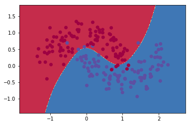
これで元記事とだいたい同じ結果が得られたと思います。