背景
神の議論を、欠損値ありデータに適用したくて、という話です。
サンプルデータ
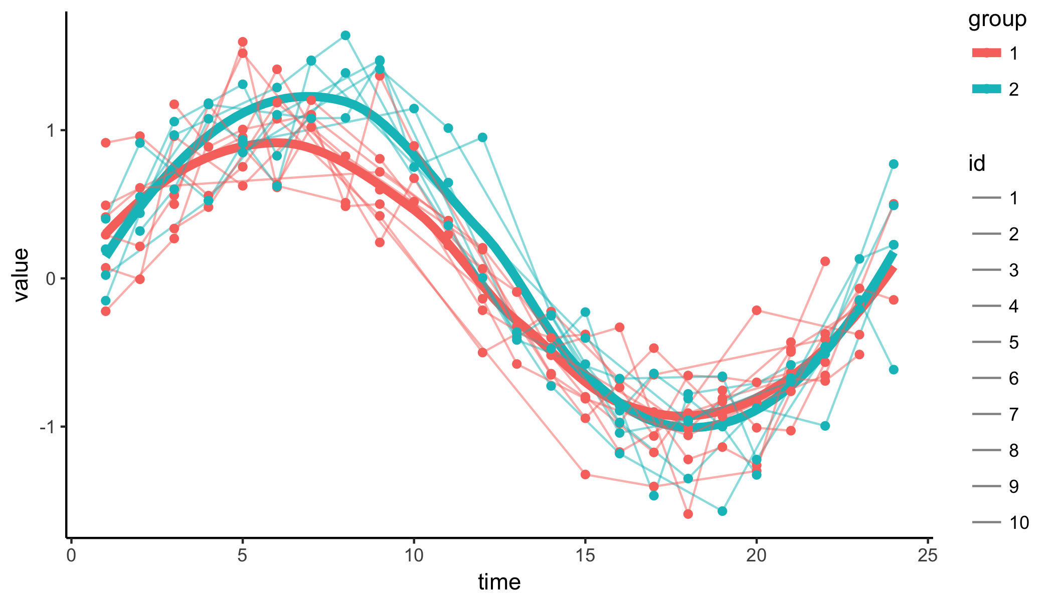
2つのグループの時系列を想定しています。
赤グループ(10系列)は、sinカーブで、sdは$0.3$です。青グループ(7系列)は、$x = 7:12$の範囲において赤よりも$0.5$だけ値が大きくなるように仕組まれています。また、データ全体は、欠損値を$50$%含んでいます。
太線は$loess$近似曲線です。
モデル
これは、神の議論のモデル2と同一です。
\begin{eqnarray}
\mu_t &\sim& normal(2*\mu_{t-1}-\mu_{t-2},σ_μ)\\
σ_t &\sim& cauchy(σ_{t-1}, σ_σ)\\
Y_{0t} &\sim& normal(\mu_t, σ_Y)\\
Y_{1t} &\sim& normal(\mu_t+σ_t, σ_Y)\\
\end{eqnarray}
stanコード
 data{
    int N_time;

    int N_sample;
    vector[N_sample] Y;
    int S[N_time];

    int N_sample1;
    vector[N_sample1] Y1;
    int S1[N_time];
  }

  parameters{
    real di0;
    vector<lower = -pi()/2, upper = pi()/2>[N_time-1] di_unif;
    real<lower = 0> s_di;

    real mu[N_time];
    real<lower = 0> s;
    real<lower = 0> s_mu;
  }

  transformed parameters{
    vector[N_time] di;
    di[1] = di0;
    for(t in 2:N_time)
      di[t] = di[t-1] + s_di * tan(di_unif[t-1]);
  }

  model{
    int pos;
    int pos1;

    for(k in 3:N_time)
      mu[k] ~ normal(2 * mu[k-1] - mu[k-2], s_mu);

    pos = 1;
    for(k in 1:N_time){
      segment(Y, pos, S[k]) ~ normal(mu[k], s);
      pos = pos + S[k];
    }

    pos1 = 1;
    for(k in 1:N_time){
      segment(Y1, pos1, S1[k]) ~ normal(mu[k] + di[k], s);
      pos1 = pos1 + S1[k];
    }
  }
前回の議論が2系列になっただけですね。$segment$を使う事で、サンプルサイズ・系列数が異なるYとY1が、どちらも$1:N_{time}$のfor文で回せている事がポイントです。
コーシー分布を使った差分の作り方は、神様のやり方を参照の事。
結果

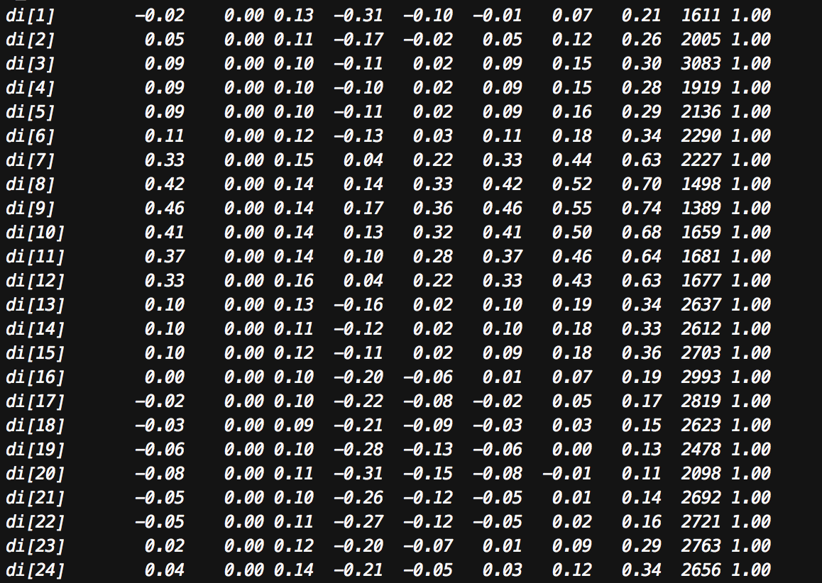
横着な結果の表示ですみません。
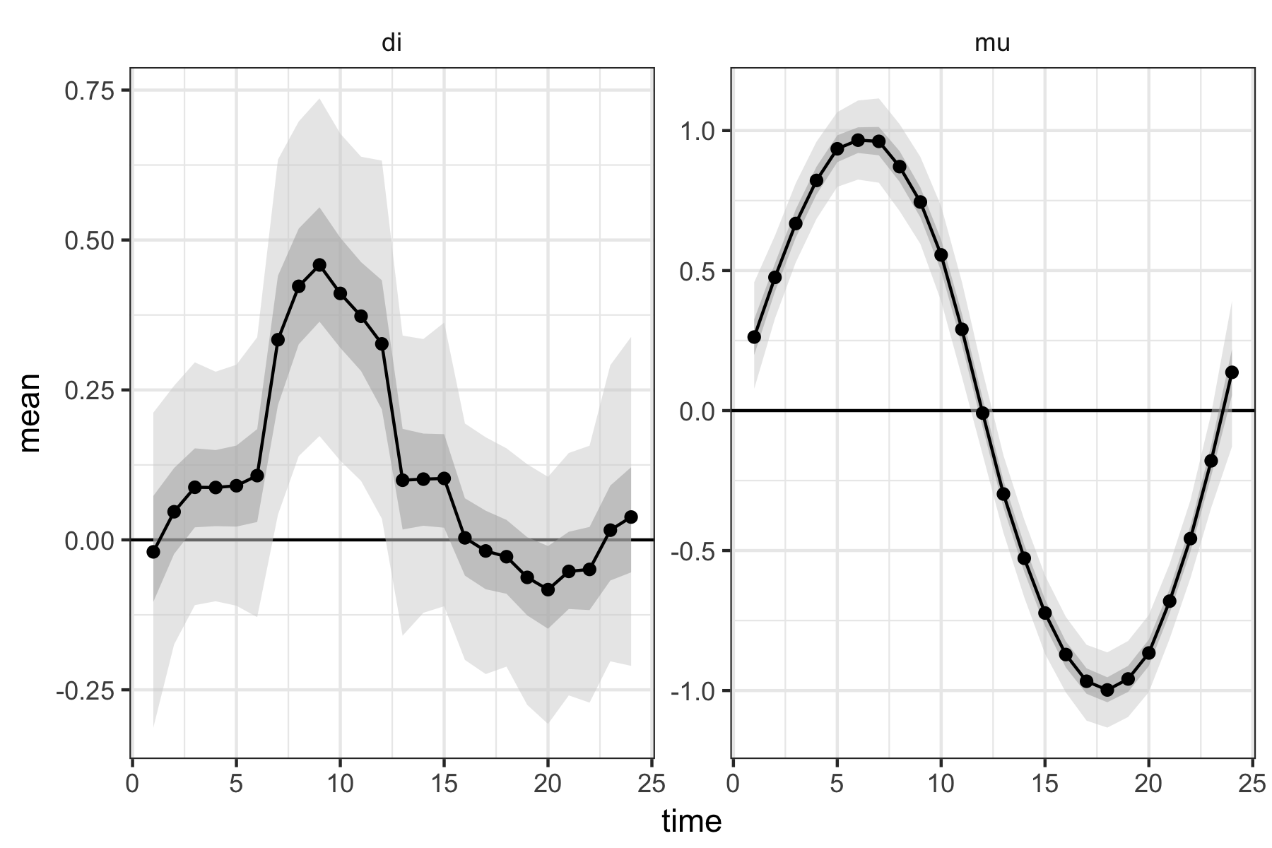
まずまずの結果ではないでしょうか。
えーと、差$di$の推定量は、$x=7:12$の範囲で、95%信用区間の下限が0を上回るため、差があると言えます。
Appendix
sample data
set.seed(123)


N_time <- 24
N_id <- 10
N_id1 <- 7
SD <- 0.3

x <- 1:N_time
y <- sin(x/N_time * 2 * pi)

Add_y <- 0.5
Add_x <- 8:12
y1 <- y
y1[Add_x] <- y1[Add_x] + Add_y

dat <- data.frame(time = x,
                  id = factor(c(rep(1:N_id, each = N_time),rep(1:N_id1, each = N_time))),
                  group = factor(c(rep(1, N_id * N_time), rep(2, N_id1 * N_time))),
                  value = c(rnorm(N_time * N_id, y, SD), rnorm(N_time * N_id1, y1, SD)))

dat1 <- dat %>%
  dplyr::mutate(index = runif(nrow(dat), 0, 1)) %>%
  dplyr::filter(index > 0.5)
Rコード
# 並列処理の指定
rstan_options(auto_write=TRUE)
options(mc.cores=parallel::detectCores())


N_time <- dat1$time  %>% factor() %>% levels() %>% length()

a <- dat1 %>% filter(group == 1) %>% arrange(time)
N_sample <- nrow(a)
Y <- a$value
S <- as.numeric(table(a$time))

a <- dat1 %>% filter(group == 2) %>% arrange(time)
N_sample1 <- nrow(a)
Y1 <- a$value
S1 <- as.numeric(table(a$time))


datastan <- list(N_time = N_time,
                 N_sample = N_sample, Y = Y, S = S,
                 N_sample1 = N_sample1, Y1 = Y1, S1 = S1)

fit <- stan(model_code = stanmodel, data = datastan, seed = 123)
お絵かき
最初の絵
ggplot(dat1, aes(time, value, color = group))+
  theme_classic()+
  geom_smooth(se = F, method = "loess", size = 2)+
  geom_path(aes(linetype = id), alpha = 0.5)+
  geom_point()+
  scale_linetype_manual(values = rep(1, N_id))
結果の絵
色々な描き方があるので、お好みで。
dat_g <- tidy(summary(fit)$summary) %>%
  filter(.rownames %in% c(paste("mu[", 1:N_time, "]", sep = ""),
                          paste("di[", 1:N_time, "]", sep = ""))) %>%
  mutate(time = as.numeric(str_sub(sapply(strsplit(.rownames, "\\["), "[[", 2), end = -2))) %>%
  mutate(label = str_sub(sapply(strsplit(.rownames, "\\["), "[[", 1), end = -1))


ggplot(dat_g, aes(x = time, y = mean))+
  theme_bw()+
  geom_hline(yintercept = 0)+
  geom_ribbon(aes(ymax = X97.5., ymin = X2.5.), fill = "lightgrey", alpha =0.5)+
  geom_ribbon(aes(ymax = X75., ymin = X25.), fill = "darkgrey", alpha =0.5)+
  geom_line()+
  geom_point()+
  facet_wrap(~label, scale = "free_y")+
  theme(strip.background = element_rect(color = "white", fill = "white"))
環境
> sessionInfo()
R version 3.3.1 (2016-06-21)
Platform: x86_64-apple-darwin13.4.0 (64-bit)
Running under: OS X 10.10.5 (Yosemite)

attached base packages:
[1] stats     graphics  grDevices utils     datasets  methods   base

other attached packages:
[1] stringr_1.2.0        broom_0.4.1          ggmcmc_1.1
[4] tidyr_0.6.0          rstan_2.14.1         StanHeaders_2.14.0-1
[7] ggplot2_2.2.1        dplyr_0.5.0
あれ?ggplot2が古いぞ?ま、いっか。