サポートベクトルマシン – Python機械学習第三章学習メモ

元記事はこちら

最近Python機械学習を読み進めているのですが、その学習メモです。
前回はこちら

SVM最適化の目的

マージンを最大化すること

• マージン：超平面（決定境界）と、この超平面に最も近いトレーニングサンプルの間の距離
• サポートベクトル：超平面に最も近いトレーニングサンプル

超平面

正の超平面

$$ w_0 + {\boldsymbol w^Tx_{pos}} = 1 $$

負の超平面

$$ w_0 + {\boldsymbol w^Tx_{neg}} = -1 $$
引き算して
$$　{\boldsymbol w^T(x_{pos} - x_{neg}}) = 2 $$
ここでベクトルの長さを以下のように定義する
$$　{\boldsymbol ||w||} = \sqrt{\sum_{j=1}^m w_j^2} $$
上2式から長さで割って標準化すると

$$　\frac{{\boldsymbol w^T(x_{pos} - x_{neg}})}{{\boldsymbol ||w||}} = \frac{2}{{\boldsymbol ||w||}} $$
左辺は正の超平面と負の超平面の距離 -> 最大化したいマージン

つまり、$　\frac{2}{{\boldsymbol ||w||}} $の最大化がマージン最大化の問題である。

正のサンプルはすべて正の超平面の後ろに収まる。
$$ w_0 + {\boldsymbol w^Tx^{(i)}} \geq 1\; \; (y^{(i)} = 1)$$
負のサンプルはすべて負の超平面の側にある。
$$ w_0 + {\boldsymbol w^Tx^{(i)}} < -1\; \; (y^{(i)} = -1)$$

実際は、$　\frac{2}{{\boldsymbol ||w||}} $の最大化ではなく逆数の二乗$　\frac{{\boldsymbol ||w||}^2}{2} $の最小化の方が簡単。二次計画法により解くことができる。

スラック変数を使った非線形分離可能なケース

スラック変数：不等式制約を等式制約に変換するために導入する変数のこと

$$ {\boldsymbol w^Tx^{(i)}} \geq 1 - \xi^{(i)}\; (y^{(i)} = 1)$$
$$ {\boldsymbol w^Tx^{(i)}} < -1 + \xi^{(i)}\; (y^{(i)} = -1)$$

最小化すべき新しい対象は下記のとおり

$$　\frac{1}{2}{\boldsymbol ||w||^2} = C\biggl({\sum_{i}\xi^{(i)}}\biggr) $$

SVMを使ったIrisデータの分類

データの準備

from sklearn import datasets
import numpy as np
from sklearn.cross_validation import train_test_split
from sklearn.preprocessing import StandardScaler
from sklearn.linear_model import Perceptron
from sklearn.metrics import accuracy_score

# Irisデータセットをロード
iris = datasets.load_iris()
# 3,4列目の特徴量を抽出
X = iris.data[:, [2, 3]]
# クラスラベルを取得
y = iris.target
# print('Class labels:', np.unique(y))

# テストデータの分離
X_train, X_test, y_train, y_test = train_test_split(X, y, test_size=0.3, random_state=0)

# 特徴量のスケーリング
sc = StandardScaler()
# トレーニングデータの平均と標準偏差を計算
sc.fit(X_train)
# 平均と標準偏差を用いて標準化
X_train_std = sc.transform(X_train)
X_test_std = sc.transform(X_test)

from sklearn.preprocessing import StandardScaler
sc = StandardScaler()
sc.fit(X_train)
X_train_std = sc.transform(X_train)
X_test_std = sc.transform(X_test)
X_combined_std = np.vstack((X_train_std, X_test_std))
y_combined = np.hstack((y_train, y_test))

プロット関数

from matplotlib.colors import ListedColormap
import matplotlib.pyplot as plt
import warnings

def versiontuple(v):
    return tuple(map(int, (v.split("."))))


def plot_decision_regions(X, y, classifier, test_idx=None, resolution=0.02):

    # setup marker generator and color map
    markers = ('s', 'x', 'o', '^', 'v')
    colors = ('red', 'blue', 'lightgreen', 'gray', 'cyan')
    cmap = ListedColormap(colors[:len(np.unique(y))])

    # plot the decision surface
    x1_min, x1_max = X[:, 0].min() - 1, X[:, 0].max() + 1
    x2_min, x2_max = X[:, 1].min() - 1, X[:, 1].max() + 1
    xx1, xx2 = np.meshgrid(np.arange(x1_min, x1_max, resolution),
                           np.arange(x2_min, x2_max, resolution))
    Z = classifier.predict(np.array([xx1.ravel(), xx2.ravel()]).T)
    Z = Z.reshape(xx1.shape)
    plt.contourf(xx1, xx2, Z, alpha=0.4, cmap=cmap)
    plt.xlim(xx1.min(), xx1.max())
    plt.ylim(xx2.min(), xx2.max())

    for idx, cl in enumerate(np.unique(y)):
        plt.scatter(x=X[y == cl, 0],
                    y=X[y == cl, 1],
                    alpha=0.6,
                    c=cmap(idx),
                    edgecolor='black',
                    marker=markers[idx],
                    label=cl)

    # highlight test samples
    if test_idx:
        # plot all samples
        if not versiontuple(np.__version__) >= versiontuple('1.9.0'):
            X_test, y_test = X[list(test_idx), :], y[list(test_idx)]
            warnings.warn('Please update to NumPy 1.9.0 or newer')
        else:
            X_test, y_test = X[test_idx, :], y[test_idx]

        plt.scatter(X_test[:, 0],
                    X_test[:, 1],
                    c='',
                    alpha=1.0,
                    edgecolor='black',
                    linewidths=1,
                    marker='o',
                    s=55, label='test set')

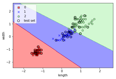
SVMで分類・表示

from sklearn.svm import SVC
svm = SVC(kernel='linear', C=1.0, random_state=0)
svm.fit(X_train_std, y_train)
plot_decision_regions(X_combined_std, y_combined, classifier=svm, test_idx=range(105,150))
plt.xlabel('length')
plt.ylabel('width')
plt.legend(loc='upper left')
plt.show()

実行結果

カーネルSVMを使って非線形問題の解を求める

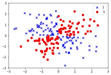
XORデータセットを作成する

np.random.seed(0)
X_xor = np.random.randn(200, 2)
y_xor = np.logical_xor(X_xor[:, 0] > 0, X_xor[:, 1] > 0)
y_xor = np.where(y_xor, 1, -1)
plt.scatter(X_xor[y_xor==1, 0], X_xor[y_xor==1, 1], c='b', marker='x', label='1')
plt.scatter(X_xor[y_xor==-1, 0], X_xor[y_xor==-1, 1], c='r', marker='s', label='-1')
plt.xlim([-3, 3])
plt.ylim([-3, 3])
plt.legend(loc='best')
plt.show()

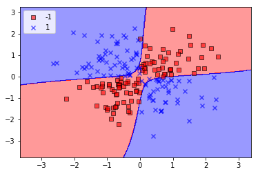
カーネルトリックを使って分離超平面を高次元空間で特定する

非線形の解は射影関数$ \phi(\cdot) $を使ってトレーニングセットをより高い次元の特徴空間に移すことで可能となる。しかし、計算コストが高いのでカーネル関数を定義する。

$$ k({\boldsymbol x^{(i)}},{\boldsymbol x^{(j)}}) = \phi({\boldsymbol x^{(i)}})^T\phi({\boldsymbol x^{(j)}}) $$

• カーネル：2つのサンプル間の「類似性を表す関数」。
• 類似度は1(全く同じ)から0(全く異なる)の間。

最も広く利用されているカーネルは動径基底関数カーネル(Radial Basis Function kernel:RBF)。ガウスカーネルとも。

$$ k({\boldsymbol x^{(i)}},{\boldsymbol x^{(j)}}) = \exp\biggl(-\frac{{||\boldsymbol x^{(i)}} - {\boldsymbol x^{(j)}}||^2}{2\sigma^2}\biggr) $$
簡略化版

$$ k({\boldsymbol x^{(i)}},{\boldsymbol x^{(j)}}) = \exp\bigl(-\gamma{||\boldsymbol x^{(i)}} - {\boldsymbol x^{(j)}}||^2\bigr) $$
$ \gamma = \frac{1}{2\sigma^2} $が最適化されるハイパーパラメータ。

# 上のコードのkernel='linear'を'rbf'に置き換える
svm = SVC(kernel='rbf', random_state=0, gamma=0.1, C=10.0)
svm.fit(X_xor, y_xor)
plot_decision_regions(X_xor,y_xor, classifier=svm)
plt.legend(loc='upper left')
plt.show()

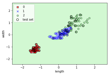
Irisデータに対してgammaを変えて適用してみる

gammaを色々変えると面白い。大きくすればするほどトレーニングデータにフィットするが、過学習になる。

svm = SVC(kernel='rbf', C=1.0, random_state=0, gamma=100)
svm.fit(X_train_std, y_train)
plot_decision_regions(X_combined_std, y_combined, classifier=svm, test_idx=range(105,150))
plt.xlabel('length')
plt.ylabel('width')
plt.legend(loc='upper left')
plt.show()