初めに

「個々の施策が売り上げにどの程度影響しているか」「個々の媒体への出稿が流入数にどの程度影響しているか」など、時系列の説明変数を用いて時系列の被説明変数を説明したい場面は多々あると思います。
また、「この施策は導入当初は効果があったが、今でも本当に効いているのか」「ユーザーは施策に飽きを感じているのではないか」など、施策の効果は時と共に変わっていくという仮定は自然な発想です。
前回はカルマンフィルタを用いて状態の推定・予測・平滑化を行いましたが、今回はカルマンフィルタを用いて係数が時変な回帰問題を解きます。

モデル

2つの説明変数$x^1, x^2$を用いて$y$を回帰する場合は、以下のようになります。

x_t = 
\begin{bmatrix}
 \alpha_t \\
 \beta_t^1 \\
 \beta_t^2 \\
\end{bmatrix}, 
G_t = I, 
F_t =
\begin{bmatrix}
 1 & x_t^1 & x_t^2
\end{bmatrix},
W =
\begin{bmatrix}
 W^{\alpha} & 0 & 0 \\
 0 & W^{\beta^1} & 0 \\
 0 & 0 & W^{\beta^2} \\
\end{bmatrix},
V = V \\
x_t = G x_{t-1} + w_t, w_t \sim N(0, W) \\
y_t = F x_t + v_t, v_t \sim N(0, V)

$I$は単位行列、Vはスカラー(値)です。
状態空間の回帰モデルでは、回帰係数が状態となります。
状態方程式(2段目の式)を見ると、状態$x_t$が遷移する度に(時点tが増えていく度に)、回帰式の切片$\alpha_t$と係数$\beta_t^1, \beta_t^2$が変わっていくのがわかります。
観測方程式(3段目の式)を見ると、観測値$y_t$は、$F x_t$、つまり$\alpha_t +\beta_t^1 x_t^1 + \beta_t^2 x_t^2$によって計算されます。

シミュレーション

ライブラリのインストール

import pandas as pd
import numpy as np
import matplotlib.pyplot as plt
import seaborn as sns
from tqdm import tqdm_notebook as tqdm

np.random.seed(1234)
pd.set_option('display.max_columns', None)
sns.set_style('darkgrid')

%matplotlib inline

仮想データの作成

T = 100
x1_diff = np.random.normal(0, 100, T)
x2_diff = np.random.normal(0, 100, T)
x1 = np.zeros(T)
x2 = np.zeros(T)
for t in range(T-1):
    x1[t+1] = 0.8 * x1[t] + x1_diff[t+1]
    x2[t+1] = 0.8 * x2[t] + x2_diff[t+1]
x1[0] = x1_diff[0]
x2[0] = x2_diff[0]
x1 += 500
x2 += 500

G = np.eye(3)
F = np.ones((T, 3))
F[:,1] = x1
F[:,2] = x2

# 状態雑音、観測雑音
W = np.diag([100, 100, 100])
V = 100
w = np.random.multivariate_normal(np.zeros(3), W, T)
v = np.random.normal(0, V, T)

# 真の係数行列
X_diff = np.random.multivariate_normal(np.zeros(3), np.diag([1000,1,1]), T)
X = np.zeros((T, 3))
for t in range(T-1):
    X[t+1] = X[t] + X_diff[t+1]
X[0] = X_diff[0]
X += np.array([1000, 0, 0])
X[:,1] *= 2

# 解釈がしづらいので、係数の最低値を正にする
for i in range(3):
    if np.min(X[:,i]) < 0:
        X[:,i] -= np.min(X[:,i])
# 観測値y
y = np.sum(F * X + w, axis=1) + v

# 仮想データをプロット
fig, axes = plt.subplots(nrows=4, figsize=(16, 8))
axes[0].plot(y, label='y')
axes[1].plot(X[:,0], label='alpha')
axes[2].plot(X[:,1], label='beta1')
axes[2].plot(X[:,2], label='beta2')
axes[3].plot(x1, label='x1')
axes[3].plot(x2, label='x2')

[axes[i].legend(loc='upper left') for i in range(4)]
plt.show()

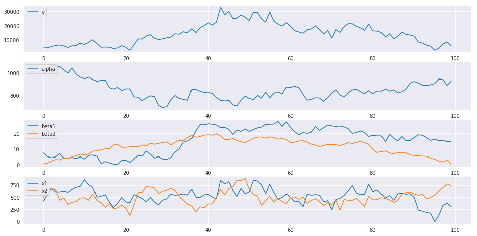
上から順に、観測値y, 切片$\alpha$, 係数$\beta^1, \beta^2$, 説明変数$x^1, x^2$となります。
$\beta^1$, $\beta^2$を見ると、時点35までは$\beta^2$の方が係数の値が大きいものの、時点35以降は$\beta^1$の方が大きいです。つまり、時点35までは$x^2$, 時点35以降は$x^1$の方が効率よく$y$に影響を与えている傾向が見えます。
しかし、実際に見ることのできる$x^1, x^2, y$だけでは、これらの傾向を読み取ることが難しいです。
そこで、カルマンフィルタを用いて未知の係数を推定します。

def kalman_filter(m, C, y, G=G, F=F, W=W, V=V):
    """
    Kalman Filter
    m: 時点t-1のフィルタリング分布の平均
    C: 時点t-1のフィルタリング分布の分散共分散行列
    y: 時点tの観測値
    Fは関数の外でわちゃわちゃやるの面倒なので、1次元で入れる
    """
    assert F.ndim == 1, print("F must be 1 dim")
    F = F.reshape(1, -1)
    a = G @ m
    R = G @ C @ G.T + W
    f = F @ a
    Q = F @ R @ F.T + V
    # 逆行列と何かの積を取る場合は、invよりsolveを使った方がいいらしい
    K = (np.linalg.solve(Q.T, F @ R.T)).T
    # K = R @ F.T @ np.linalg.inv(Q)
    m = a + K @ (y - f)
    C = R - K @ F @ R
    return m, C, a, R, f, Q

def kalman_smoothing(s, S, m, C, a, R, G=G, W=W):
    """
    Kalman smoothing
    """
    # 平滑化利得の計算
    A = np.linalg.solve(R, C @ G.T)
    # A = C @ G.T @ np.linalg.inv(R)
    # 状態の更新
    s = m + A @ (s - a)
    S = C + A @ (S - R) @ A.T
    return s, S

推定

# 結果を格納するarray
m_result = np.zeros((T, 3))
C_result = np.zeros((T, 3, 3))
a_result = np.zeros((T, 3))
R_result = np.zeros((T, 3, 3))
f_result = np.zeros((T))
Q_result = np.zeros((T))
s_result = np.zeros((T, 3))
S_result = np.zeros((T, 3, 3))

m0 = np.zeros(3)
C0 = np.diag([1e8]*3)

for t in range(T):
    if t == 0:
        m_result[t], C_result[t], a_result[t], R_result[t], f_result[t], Q_result[t] = kalman_filter(m0, C0, y[t], F=F[t])
    else:
        m_result[t], C_result[t], a_result[t], R_result[t], f_result[t], Q_result[t] = kalman_filter(m_result[t-1], C_result[t-1], y[t], F=F[t])

for t in range(T):
    t = T - t - 1
    if t == T - 1:
        s_result[t], S_result[t] = m_result[t], C_result[t]
    else:
        s_result[t], S_result[t] = kalman_smoothing(s_result[t+1], S_result[t+1], m_result[t], C_result[t], a_result[t+1], R_result[t+1], W=W)

結果の描画

fig, axes = plt.subplots(nrows=3, figsize=(16, 6))
axes[0].plot(X[:,1], label='beta1')
axes[0].plot(X[:,2], label='beta2')
axes[1].plot(s_result[:,1], label='beta1')
axes[1].plot(s_result[:,2], label='beta2')
axes[2].plot(X[:,0], label="real")
axes[2].plot(s_result[:,0], label="predict")

axes[0].legend(loc=loc)
axes[1].legend(loc=loc)
axes[2].legend(loc=loc)

axes[0].set_title("beta1 vs beta2 real")
axes[1].set_title("beta1 vs beta2 predict")
axes[2].set_title("alpha")

plt.show()

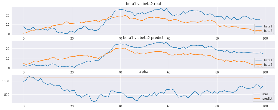
真の係数比較図をそれなりに復元出来ている事がわかります。
この結果を用いれば、例えば$x^2$は効率が悪いので$x_1$の配分を増やす、といった施策に結びつける事が出来ます。
一方で、切片$\alpha$は上手く復元出来ませんでした。何となく難しそうではありますが、ちょっとわからないので色々考えてみます。

まとめ

カルマンフィルタを用いて時系列データに対する回帰問題を解いた
複数の説明変数について、時と共に変わる係数を推定した
個々の説明変数がどれくらい被説明変数に対して影響を与えているのか推定出来る

カルマンフィルタを使って時系列に対する回帰問題を解く

初めに

モデル

シミュレーション

まとめ