クロスバリデーションとグリッドサーチ(備忘録)

このブログについて

• 備忘録のためにクロスバリデーション、及びグリットサーチについてまとめます
• Pythonのscikit-learnライブラリを使用します

クロスバリデーション

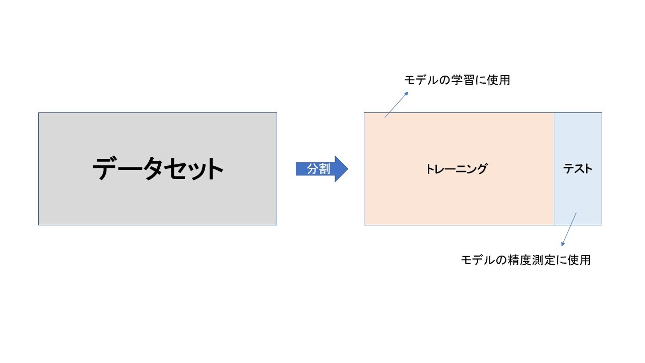
トレーニングデータとテストデータへの分割

機械学習では過学習を避けるため、及び未知のデータへの予測精度を検証するため、与えられたデータセットを訓練用データと検証用データに分割します。

scikit-learnのデータセットを使ってデータの分割を行います

from sklearn.datasets import load_wine
from sklearn.model_selection import train_test_split

# datasetのインスタンスを宣言
wine = load_wine()
#　説明変数と目的変数を生成
X = wine.data
y = wine.target
# データを分割
X_train, X_test, y_train, y_test = train_test_split(X, y, random_state=0)
'''
[out]
データセットのレコード数:  178 
トレーニングデータのレコード数:  133 
テストデータのレコード数:  45
'''
print('データセットのレコード数: ', len(X), '\n',
      'トレーニングデータのレコード数: ', len(X_train), '\n',
      'テストデータのレコード数: ', len(X_test))

このデータを使ってモデル（今回はランダムフォレスト）の作成を行います

import numpy as np
from sklearn.ensemble import RandomForestClassifier

# パラメータは一先ず仮置き
depth = 3
leaf = 5
forest = RandomForestClassifier(n_estimators=10, max_depth=depth, min_samples_leaf=leaf).fit(X_train, y_train)

# テストデータを使ったモデルの検証
score = forest.score(X_test, y_test)

# out[score depth3 leaf5:  1.000]
print('score depth{} leaf{}:  {:0.3f}'.format(depth, leaf, score))

クロスバリデーションの実装

上の例ではscikit-learnのtrain_test_splitを使ってデータの分割を行いました。しかし、上記の結果だとトレーニングデータとテストデータの分割に、偏りが出た場合、精度検証に思ってもみないバイアスが生まれる可能性もあります。そこでクロスバリデーションという方法を使います。

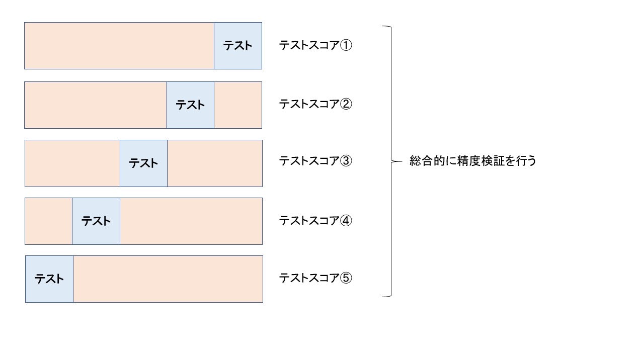
上図のように与えられたデータセットを$n$個に分割して（上記の場合は５つ）、そのうち一つをテストデータとして検証します。その処理を$n$回行うことで、モデルの精度を検証します。

from sklearn.model_selection import cross_val_score
# 桁数を指定
np.set_printoptions(precision=3)

# cv=5で分割数を指定
scores = cross_val_score(forest, X, y, cv=5)

# out[0.757  0.972  0.944  1.    0.971]
print(scores)

この場合、トレーニングとテストの分割を変えることで、精度が大きく変わってくることが確認できます

グリッドサーチ

モデルの精度を向上させるために用いられる手法で、全てのパラメータの組み合わせを試してみる方法のことです

グリッドサーチの実装

# パラメータのリストを生成
depth = [2, 3, 4, 5, 6, 7]
leaf = [1, 3, 5, 7, 12]
scores = {}

for i in depth:
    for j in leaf:
        forest =  RandomForestClassifier(n_estimators=10, max_depth=i, min_samples_leaf=j, random_state=0).fit(X_train, y_train)
        score = forest.score(X_test, y_test)
        scores['depth{}, leaf{}'.format(i, j)] = round(score, 3)

'''
[out]
{'depth2, leaf1': 0.956, 'depth2, leaf3': 0.933, 'depth2, leaf5': 0.956, 'depth2, leaf7': 0.933, 'depth2, leaf12': 0.889,
'depth3, leaf1': 0.978, 'depth3, leaf3': 0.956, 'depth3, leaf5': 0.956, 'depth3, leaf7': 0.933, 'depth3, leaf12': 0.956,
'depth4, leaf1': 0.956, 'depth4, leaf3': 1.0, 'depth4, leaf5': 0.956, 'depth4, leaf7': 0.956, 'depth4, leaf12': 0.956,
'depth5, leaf1': 0.956, 'depth5, leaf3': 1.0, 'depth5, leaf5': 0.956, 'depth5, leaf7': 0.956, 'depth5, leaf12': 0.956,
'depth6, leaf1': 0.956, 'depth6, leaf3': 1.0, 'depth6, leaf5': 0.956, 'depth6, leaf7': 0.956, 'depth6, leaf12': 0.956,
'depth7, leaf1': 0.956, 'depth7, leaf3': 1.0, 'depth7, leaf5': 0.956, 'depth7, leaf7': 0.956, 'depth7, leaf12': 0.956}
'''
print(scores)

• 上記方法を使うと、テストデータ（X_test）に対して最も当てははりの良いパラメータ、及びその時のスコアが見つかります
• しかし、実際は検証用として使うべきテストデータをチューニングに使ってモデルを構築してしまっています

学校のテストで例えると…

• 本来であれば、トレーニングデータ（学習用の参考書）を使って勉強し、本番のテスト（テストデータ）で学習成果を測るといった流れが無視されています
• 本番用のテストをカンペして、学習しているような状況になり、どれほど汎化性能の良いモデルができたのか、いまいち分からない状況になっています

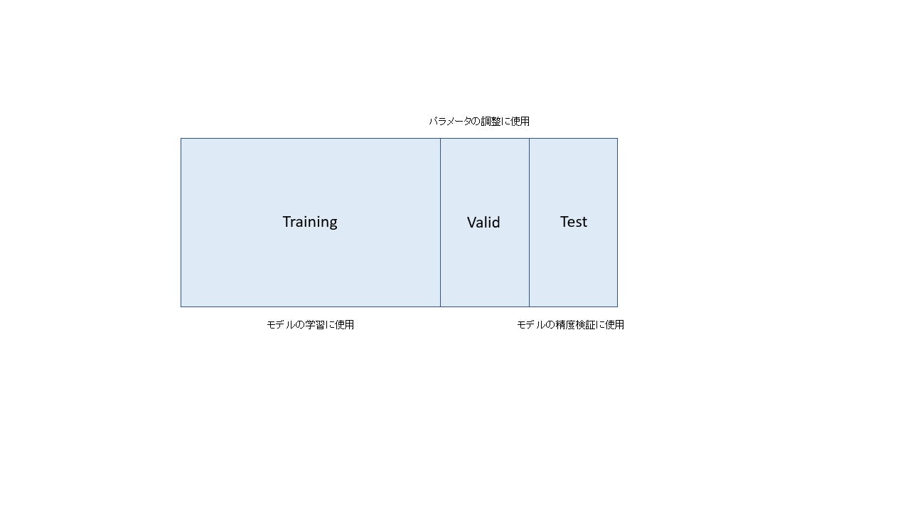
この問題を解決するため、トレーニングデータを更に学習データと、パラメータ調整用のデータに分割します。イメージは以下の通りです

X_train_val, X_test, y_train_val, y_test = train_test_split(X, y, random_state=0)

X_train, X_val, y_train, y_val = train_test_split(X_train_val, y_train_val, random_state=0)

'''
[out]
X_test shape:  (45, 13) 
X_val shape:  (34, 13) 
X_train shape:  (99, 13)
'''
print('X_test shape: ', X_test.shape, '\n'
      'X_val shape: ', X_val.shape, '\n'
      'X_train shape: ', X_train.shape)

depth = [2, 3, 4, 5, 6, 7]
leaf = [1, 3, 5, 7, 10]
best_val_score = 0   # best_scoreを初期化
best_param = {}   # best_paramを初期化

for i in depth:
    for j in leaf:
        forest = RandomForestClassifier(n_estimators=10, max_depth=i, min_samples_leaf=j, random_state=0).fit(X_train, y_train)
        score = forest.score(X_val, y_val)
        if score > best_val_score:
            best_val_score = score
            best_param = {'max_depth': i, 'min_samples_leaf': j}

'''
[out]
best_val_score:  0.941
best_param:  {'max_depth': 5, 'min_samples_leaf': 1}
'''
print('best_val_score: ', round(best_val_score, 3))
print('best_param: ', best_param)

# テストデータで精度を検証
# 引数として辞書型の前に**を持ってくることで、展開が可能
forest = RandomForestClassifier(n_estimators=10, random_state=0, **best_param).fit(X_train_val, y_train_val)
best_score = forest.score(X_test, y_test)
# [out]  best_score: 0.956
print('best_score:', round(best_score, 3))

クロスバリデーションとグリッドサーチの併用

• 計算量は大きくなってしまいますが、クロスバリデーションとグリッドサーチを併用することで最良のパラメーターを求める手法もあります
• これを交差検証法と言います

depth = [2, 3, 4, 5, 6, 7]
leaf = [1, 3, 5, 7, 10]
best_val_score = 0
best_param = {}

for i in depth:
    for j in leaf:
        forest = RandomForestClassifier(n_estimators=10, max_depth=i, min_samples_leaf=j, random_state=0)
        scores = cross_val_score(forest, X_train_val, y_train_val, cv=5)
        mean_score = np.mean(scores)
        if mean_score > best_val_score:
            best_val_score = mean_score
            best_param = {'max_depth': i, 'min_samples_leaf': j}

# out[best_val_score: 0.955]
# out[best_param:  {'max_depth': 2, 'min_samples_leaf': 1}]
print('best_val_score: {:0.3f}'.format(best_val_score))
print('best_param: ', best_param)

この手法はscikit-learnのクラスを使うことで、より少ないコードで実装できます

from sklearn.model_selection import GridSearchCV
from sklearn.ensemble import RandomForestClassifier

param_grid = {'max_depth': [2, 3, 4, 5, 6, 7],
              'min_samples_leaf': [1, 3, 5, 7, 10]}

forest = RandomForestClassifier(n_estimators=10, random_state=0)
grid_search = GridSearchCV(forest, param_grid, iid=True, cv=5, return_train_score=True)

# GridSearchCVは最良パラメータの探索だけでなく、それを使った学習メソッドも持っています
grid_search.fit(X_train_val, y_train_val)


'''
[out]
best score: 0.956
best params: {'max_depth': 2, 'min_samples_leaf': 1}
best val score:  0.955
'''
print('best score: {:0.3f}'.format(grid_search.score(X_test, y_test)))
print('best params: {}'.format(grid_search.best_params_))
print('best val score:  {:0.3f}'.format(grid_search.best_score_))

best val scoreは一つ上のコードと同じ結果になっていることが分かります

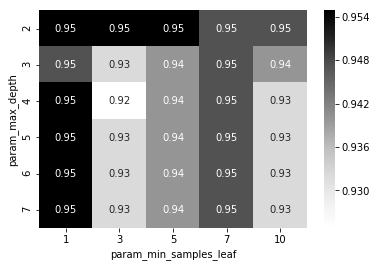
GridSearchCV結果の可視化

• GridSearchCVの結果はcv_resultというオプションを参照すれば出てきます
• 今回はpandasのデータフレーム 、及びヒートマップを使って結果の可視化を行います

import pandas as  pd
import seaborn as sns
%matplotlib inline

cv_result = pd.DataFrame(grid_search.cv_results_)
cv_result = cv_result[['param_max_depth', 'param_min_samples_leaf', 'mean_test_score']]
cv_result_pivot = cv_result.pivot_table('mean_test_score', 'param_max_depth', 'param_min_samples_leaf')

heat_map = sns.heatmap(cv_result_pivot, cmap='Greys', annot=True);

追記（2021/09/27）

　プロ野球データの可視化サイト を作りました。まだまだクオリティは低いですが、今後少しずつバージョンアップさせていく予定です。野球好きの方は是非遊びに来てください⚾️