今回のブログについて

線形代数の特異値分解についてまとめてみました
理論部分については、まだ分かっていない部分も多いので、今回は実装メインで特異値分解の様子をみていきたいと思います

特異値分解(singular value decomposition: SVD)とは

$m×n$ ($m$行$n$列)の行列を分解する方法の一つ。この時行列は正方である必要はありません
機械学習では主に次元削減に用いられます
行列$A$($m$行$n$列)を特異値分解した際の式を表すと、以下のようになります

$A = U\sum{V^T}$

$U$は$m$行$m$列の正方行列であり、更に行列式が1の直交行列である
$V^T$は$n$行$n$列の正方行列であり、更に行列式が1の直交行列である
$\sum$は「非対角成分が 0となり，対角成分は非負で大きさの順に並んだ行列」となる

A = (\begin{array}　\boldsymbol{u_1}&\boldsymbol{u_2}&\cdots&\boldsymbol{u_m} \end{array}) \begin{pmatrix}
\sigma_1  \\
              & \sigma_2 \\
              &               & \sigma_3 \\
             &                &          & \ddots \\
\end{pmatrix}
\begin{pmatrix}
\boldsymbol{v_1^T} \\
\boldsymbol{v_2^T} \\
\vdots \\
\boldsymbol{v_n^T} \\
\end{pmatrix}

具体例

\begin{pmatrix}
2 & 2 & 2 & 2 \\
1 & -1 & 1 & -1 \\
-1 & 1 & -1 & 1 \\
\end{pmatrix} = \begin{pmatrix}
1 & 0 & 0 \\
0 & -\frac{1}{\sqrt{2}} & \frac{1}{\sqrt{2}} \\
0 & \frac{1}{\sqrt{2}} & \frac{1}{\sqrt{2}}  \\
\end{pmatrix}
\begin{pmatrix}
4 & 0 & 0 & 0 \\
0 & 2\sqrt{2} & 0 & 0 \\
0 & 0 & 0 & 0 \\
\end{pmatrix}
\begin{pmatrix}
\frac{1}{2} & -\frac{1}{2} & 0 & -\frac{1}{\sqrt{2}} \\
\frac{1}{2} & \frac{1}{2} & -\frac{1}{\sqrt{2}} & 0 \\
\frac{1}{2} & -\frac{1}{2} & 0 & \frac{1}{\sqrt{2}} \\
\frac{1}{2} & \frac{1}{2} & \frac{1}{\sqrt{2}} & 0 \\
\end{pmatrix}

Pythonでの特異値分解は、numpyを使って計算できます

import numpy as np

A = np.array([[2, 2, 2, 2], [1, -1, 1, -1], [-1, 1, -1, 1]])
u, s, v = np.linalg.svd(A)

A が与えられたとき，特異値を定める行列 Σ は一意に決まりますが，直交行列 U,V は一意に定まるとは限りません
行列の特異値の数は，その行列のランクと一致します
行列の特異値の二乗和はその行列の全成分の二乗和と等しくなります

低ランク近似

$A=U\sum{}V^T$ において$\sum$は対角行列のため、対角要素σ（特異値）が大きければ、Aに与える影響も大きくなります
そこでσ（特異値）の値が小さな部分について、その行と列成分を削除した新たなSを用いて、近似することができます
低次元の行列で近似することで、次元圧縮が可能になります

import matplotlib.pyplot as plt
import seaborn as sns
%matplotlib inline

# 0から１の値を取る、10×１5の行列を作成
A = np.random.randint(0, 2, 150).reshape(10, 15)
plt.figure()
sns.heatmap(A, cmap='gray', square=True, xticklabels='', yticklabels='');

この行列を特異値分解し、ランク3で近似したいと思います。

from scipy import linalg

u, s, v = np.linalg.svd(A)

# u の先頭1列のみスライシング
ur = u[:, :3]

# 3番目までの特徴量を抽出し、　3×3の行列を生成
sr = np.matrix(linalg.diagsvd(s[:3], 3, 3))

# u の先頭1行のみスライシング
vr = v[:3, :]

'''
[out]
 u.shape:  (10, 10) 
 s.shape:  (10,) 
 v.shape:  (15, 15) 
 ur.shape:  (10, 3) 
 sr.shape:  (3, 3) 
 vr.shape:  (3, 15) 
'''
print('u.shape: ', u.shape,'\n',
       's.shape: ',  s.shape, '\n',
       'v.shape: ', v.shape, '\n',
       'ur.shape: ', ur.shape, '\n',
       'sr.shape: ', sr.shape, '\n',
       'vr.shape: ', vr.shape, '\n')

# 行列の積を求める
A_kinji = ur @ sr @ vr

sns.heatmap(A_kinji, vmin=0, vmax=1, cmap='gray', square=True, xticklabels='', yticklabels='');

元の行列に近い値を取っていることが分かります

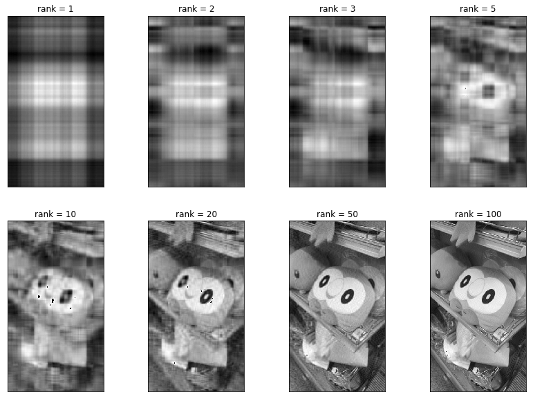
次に実際の画像を使って確認してみます(環境はJupyterNotebookです)

from PIL import Image

img = Image.open('picture.jpg')
gray_img = img.convert('L')
gray_img.save('gray_picture.jpg')
gray_img

# 特異値分解を行う関数を定義
def perform_svd(a, rank):
    u, s, v = linalg.svd(a)
    ur = u[:, :rank]
    sr = np.matrix(linalg.diagsvd(s[:rank], rank, rank))
    vr = v[:rank, :]
    return np.array(ur @ sr @ vr)

rank = [1, 2, 3, 5, 10, 20, 50, 100]


for i in rank:
    B = perform_svd(gray_img, i)
    # fromarray: NumpyのarrayからPILへの変換
    # Numpy.unit8: 8ビットの符号なし整数へ変換
    img2 = Image.fromarray(np.uint8(B))
    img2.save('gray_picture_r{}.jpg'.format(i))

gray_pic_dict = {}
index = 0

for i in rank:
    gray_pic_dict[index] = 'gray_picture_r{}.jpg'.format(i)
    index +=1

fig, axes = plt.subplots(2, 4, figsize=(14, 10), subplot_kw={'xticks': (), 'yticks': ()})

for i in range(8):
    img = Image.open(gray_pic_dict[i])
    gray_img_r_stop = img.convert('L')
    axes[i//4][i%4].imshow(gray_img_r_stop, cmap='gray')
    axes[i//4][i%4].set_title('rank = {}'.format(rank[i]))

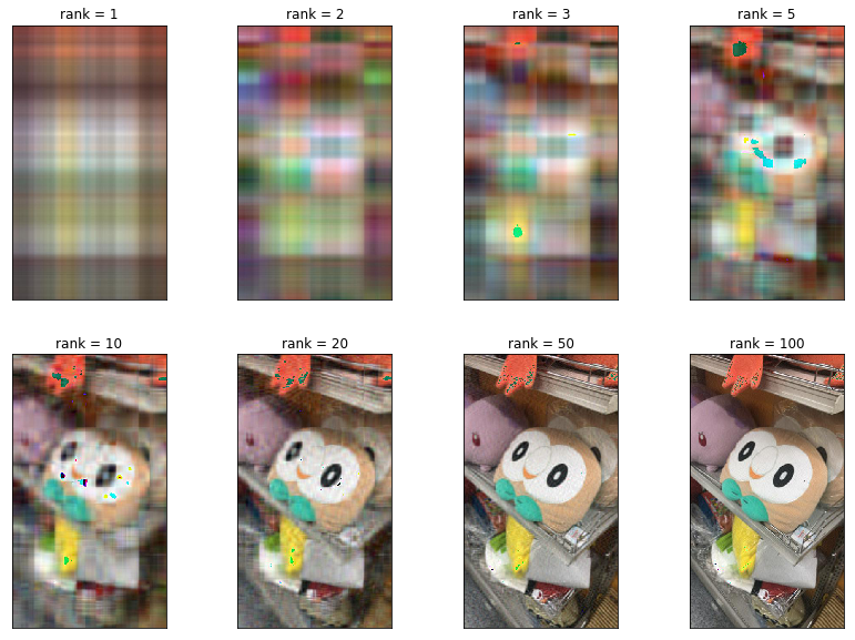
カラー画像でもやってみます。カラーの場合、単純な行列ではなく、三層のテンソルなので計算に工夫が必要です

img = Image.open('picture.jpg')
color_img = img.convert('RGB')
color_img.save('color_picture.jpg')
color_img

rank = [1, 2, 3, 5, 10, 20, 50, 100]
w = img.width
h = img.height
A = np.array(color_img)

# out[A.shape:  (640, 360, 3)]
print('A.shape: ', A.shape)
# 縦640×横360×３層のNumpy array

for i in rank:
    # 各層を特異値分解後、1次元のアレイに変換
    r = perform_svd(A[:, :, 0] ,i).reshape(w * h)
    g = perform_svd(A[:, :, 1] ,i).reshape(w * h)
    b = perform_svd(A[:, :, 2] ,i).reshape(w * h)
    # 3×(640*360)　→ (640*360)×3 → 640×360×3
    B = np.array([r,g,b]).transpose(1, 0).reshape(h, w, 3)
    img2 = Image.fromarray(np.uint8(B))
    img2.save('color_picture_r{}.jpg'.format(i))

color_pic_dict = {}
index = 0

for i in rank:
    color_pic_dict[index] = 'color_picture_r{}.jpg'.format(i)
    index +=1

fig, axes = plt.subplots(2, 4, figsize=(14, 10), subplot_kw={'xticks': (), 'yticks': ()})

for i in range(8):
    img = Image.open(color_pic_dict[i])
    color_img_r_stop = img.convert('RGB')
    axes[i//4][i%4].imshow(color_img_r_stop)
    axes[i//4][i%4].set_title('rank = {}'.format(rank[i]))

追記（2021/09/27）

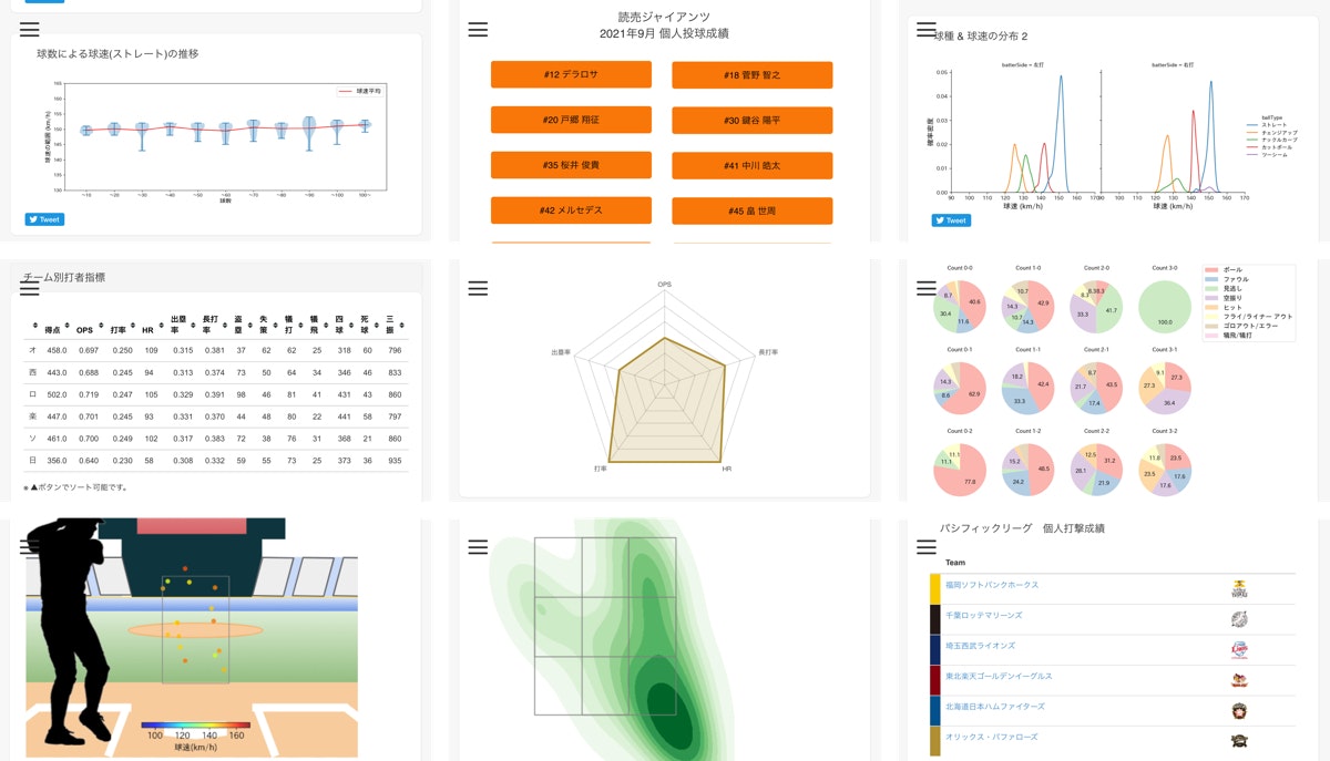
　プロ野球データの可視化サイトを作りました。まだまだクオリティは低いですが、今後少しずつバージョンアップさせていく予定です。野球好きの方は是非遊びに来てください⚾️

特異値分解による低ランク近似

今回のブログについて

特異値分解(singular value decomposition: SVD)とは

具体例

低ランク近似

追記（2021/09/27）