LSTMを使用した株価予測サンプルをPython3で実行

概要

LSTMを使用した株価予測サンプルをかなり前に試してみたのですが
放置状態なっていたので、忘れないうちにメモを残しておきます。

※参考元はPython2系、ipynb形式ですが
　今回はPython3系、py形式で動かせるように修正し試しました

・環境情報
Windows10 Pro
Anaconda 1.9.X
Python 3.6.X
keras 2.2.4
numpy 1.15.4

Visual studio Code

実施手順

１．実施環境

下記はインストール済みであることが前提
Anaconda1.9.X
Python 3.6.X
keras 2.2.4
numpy 1.15.4

実行アプリは以下を使用
Visual studio Code

２．学習アプリの準備

以下URLから「Clone or Download」をクリックし「How-to-Predict-Stock-Prices-Easily-Demo-master.zip」をダウンロード
https://github.com/llSourcell/How-to-Predict-Stock-Prices-Easily-Demo
上記ダウンロードファイルを解凍し、フォルダを任意の場所に配置

上記解凍フォルダに以下の２つのソースコード「stockdemo.py」「lstm.py」を置く
※Python2.X系、Jupyter Notebook の場合は「stockdemo.ipynb」で実行できるはず？

stockdemo.py

from keras.layers.core import Dense, Activation, Dropout
from keras.layers.recurrent import LSTM
from keras.models import Sequential
import lstm, time #helper libraries

#Step 1 Load Data
X_train, y_train, X_test, y_test = lstm.load_data('sp500.csv', 50, True)

#Step 2 Build Model
model = Sequential()

model.add(LSTM(
    input_dim=1,
    output_dim=50,
    return_sequences=True))
model.add(Dropout(0.2))

model.add(LSTM(
    100,
    return_sequences=False))
model.add(Dropout(0.2))

model.add(Dense(
    output_dim=1))
model.add(Activation('linear'))

start = time.time()
model.compile(loss='mse', optimizer='rmsprop')
print('compilation time : ', time.time() - start)

#Step 3 Train the model
model.fit(
    X_train,
    y_train,
    batch_size=512,
    nb_epoch=1,
    validation_split=0.05)

#Step 4 - Plot the predictions!
predictions = lstm.predict_sequences_multiple(model, X_test, 50, 50)
lstm.plot_results_multiple(predictions, y_test, 50)

lstm.py

import time
import warnings
import numpy as np
from numpy import newaxis
from keras.layers.core import Dense, Activation, Dropout
from keras.layers.recurrent import LSTM
from keras.models import Sequential
import matplotlib.pyplot as plt


warnings.filterwarnings("ignore")

def plot_results_multiple(predicted_data, true_data, prediction_len):
    fig = plt.figure(facecolor='white')
    ax = fig.add_subplot(111)
    ax.plot(true_data, label='True Data')
    print('yo')
    #Pad the list of predictions to shift it in the graph to it's correct start
    for i, data in enumerate(predicted_data):
        padding = [None for p in range(i * prediction_len)]
        plt.plot(padding + data, label='Prediction')
        plt.legend()
    plt.show()

def load_data(filename, seq_len, normalise_window):
    f = open(filename, 'r').read()
    data = f.split('\n')

    sequence_length = seq_len + 1
    result = []
    for index in range(len(data) - sequence_length):
        result.append(data[index: index + sequence_length])

    if normalise_window:
        result = normalise_windows(result)

    result = np.array(result)

    row = round(0.9 * result.shape[0])
    train = result[:int(row), :]
    np.random.shuffle(train)
    x_train = train[:, :-1]
    y_train = train[:, -1]
    x_test = result[int(row):, :-1]
    y_test = result[int(row):, -1]

    x_train = np.reshape(x_train, (x_train.shape[0], x_train.shape[1], 1))
    x_test = np.reshape(x_test, (x_test.shape[0], x_test.shape[1], 1))  

    return [x_train, y_train, x_test, y_test]

def normalise_windows(window_data):
    normalised_data = []
    for window in window_data:
        normalised_window = [((float(p) / float(window[0])) - 1) for p in window]
        normalised_data.append(normalised_window)
    return normalised_data

def build_model(layers):
    model = Sequential()

    model.add(LSTM(
        input_dim=layers[0],
        output_dim=layers[1],
        return_sequences=True))
    model.add(Dropout(0.2))

    model.add(LSTM(
        layers[2],
        return_sequences=False))
    model.add(Dropout(0.2))

    model.add(Dense(
        output_dim=layers[3]))
    model.add(Activation("linear"))

    start = time.time()
    model.compile(loss="mse", optimizer="rmsprop")
    print("Compilation Time : ", time.time() - start)
    return model

def predict_point_by_point(model, data):
    #Predict each timestep given the last sequence of true data, in effect only predicting 1 step ahead each time
    predicted = model.predict(data)
    predicted = np.reshape(predicted, (predicted.size,))
    return predicted

def predict_sequence_full(model, data, window_size):
    #Shift the window by 1 new prediction each time, re-run predictions on new window
    curr_frame = data[0]
    predicted = []
    for i in range(len(data)):
        predicted.append(model.predict(curr_frame[newaxis,:,:])[0,0])
        curr_frame = curr_frame[1:]
        curr_frame = np.insert(curr_frame, [window_size-1], predicted[-1], axis=0)
    return predicted

def predict_sequences_multiple(model, data, window_size, prediction_len):
    #Predict sequence of 50 steps before shifting prediction run forward by 50 steps
    prediction_seqs = []
    for i in range((int)(len(data)/prediction_len)):
        curr_frame = data[i*prediction_len]
        predicted = []
        for j in range(prediction_len):
            predicted.append(model.predict(curr_frame[newaxis,:,:])[0,0])
            curr_frame = curr_frame[1:]
            curr_frame = np.insert(curr_frame, [window_size-1], predicted[-1], axis=0)
        prediction_seqs.append(predicted)
    return prediction_seqs

３．実行と結果確認

stockdemo.pyを実行すると、以下のように結果がグラフで表示される

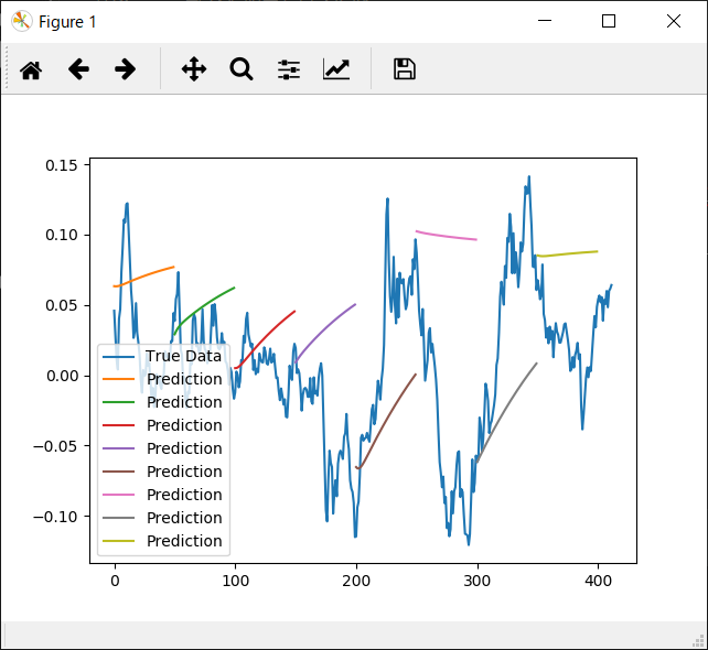
※predictionとなっているところが、LSTMによる予測

以上

参考文献
https://futurismo.biz/archives/6389/
https://github.com/llSourcell/How-to-Predict-Stock-Prices-Easily-Demo

python V2→V3差分修正
http://diveintopython3-ja.rdy.jp/porting-code-to-python-3-with-2to3.html