0.概要
CNNを用いて心電図の1拍分の波形から不整脈を分類します。(参考論文で紹介されていたモデルの実験的な実装です。実用性等は考えていないのでモデルのチューニングや比較検証はしません。)
1.不整脈とECG
不整脈
正常な心臓の拍動を「洞調律(サイナス)」と言い、不整脈とは文字通り脈が不整になることで、拍動が遅くなったり早くなったり乱れたりします。それぞれを「徐脈性不整脈」、「頻脈性不整脈」、「期外収縮」と言います。筋肉は支配神経からの電気的信号を元に運動するので、電位変化を記録することで筋肉の運動を把握できます。心電図(ECG)は心筋の筋電図であり、何らかの原因によって心筋に異常が生じるとECGにその影響が現れます。今回はECGの1拍分のデータを用いて機械学習で不整脈の分類をしてみます。(詳しくは[1]の参考書が分かりやすいです。)
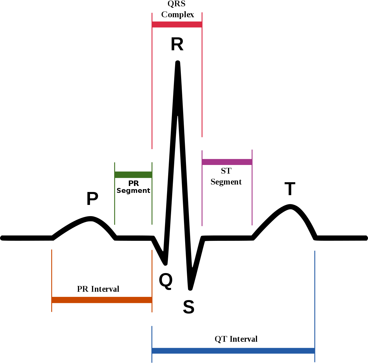
図1.1 洞調律の波形(Wikipedia)
Dataset
- Python: 3.6.7
用いるのはMIT-BIHのECGデータ1拍分[2]でKaggleからダウンロードできます。データは前処理されていて、5つのクラスに分けられています。
0: N, 1: S, 2: V, 3: F, 4: Q
それぞれのクラスに以下のようにいくつかの不整脈が含まれます。
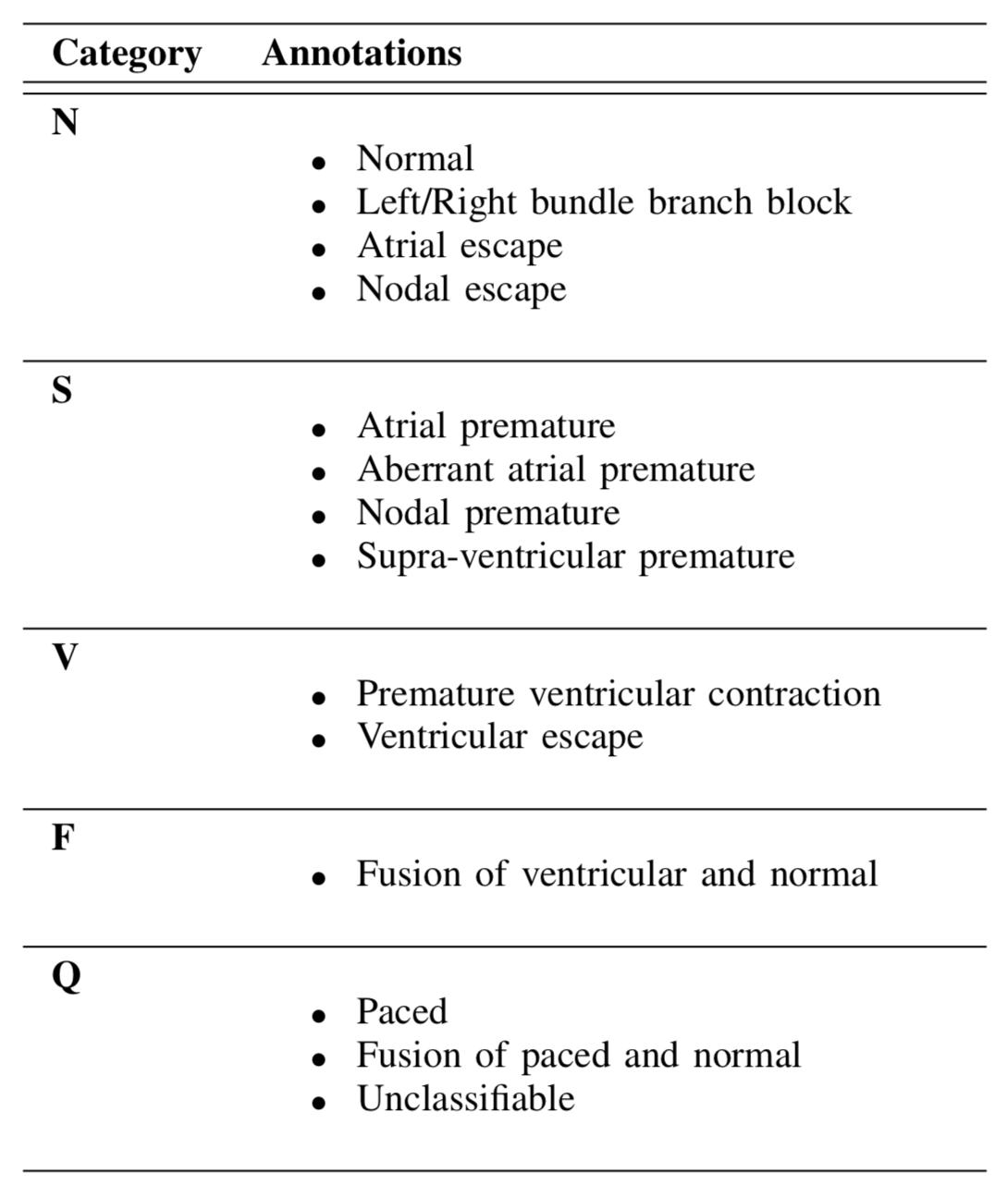
図1.2 クラス分類
各クラスのデータ数は、
Code
import numpy as np
import pandas as pd
import matplotlib.pyplot as plt
import seaborn as sns
import time
import copy
import torch
import torch.nn as nn
from torch.utils.data import Dataset, DataLoader, random_split
from torch.optim import Adam
from torch.optim.lr_scheduler import ReduceLROnPlateau
from sklearn.metrics import f1_score, confusion_matrix, roc_curve, auc
import warnings
warnings.filterwarnings('ignore')
plt.style.use('default')
sns.set()
sns.set_style('whitegrid')
train_df = pd.read_csv("./mitbih_train.csv")
test_df = pd.read_csv("./mitbih_test.csv")
print('Train data')
print(train_df.info())
print('Type Count')
print(train_df.iloc[:, 187].value_counts())
print('--------------------')
print('Test data')
print(test_df.info())
print('Type Count')
print(test_df.iloc[:, 187].value_counts())
| Class | 0 | 1 | 2 | 3 | 4 |
|---|---|---|---|---|---|
| Train | 72471 | 2223 | 5788 | 641 | 6431 |
| Test | 18118 | 556 | 1448 | 162 | 1608 |
各クラスの心電図は下の図のようになります。
Code
train_X = train_df.values[:, :-1]
train_y = train_df.values[:, -1].astype(int)
test_X = test_df.values[:, :-1]
test_y = test_df.values[:, -1].astype(int)

train_X = np.concatenate([train_X, np.zeros((train_X.shape[0], 5))], axis=1)
test_X = np.concatenate([test_X, np.zeros((test_X.shape[0], 5))], axis=1)

train_y_onehot = np.zeros((train_X.shape[0], 5))
for i in range(train_X.shape[0]):
    train_y_onehot[i, train_y[i]] = 1
test_y_onehot = np.zeros((test_X.shape[0], 5))
for i in range(test_X.shape[0]):
    test_y_onehot[i, test_y[i]] = 1

x = np.arange(0, 192)*8/1000
classes = ['N', 'S', 'V', 'F', 'Q']

fig = plt.figure(figsize=(8, 16))
ax1 = fig.add_subplot(511)
ax2 = fig.add_subplot(512)
ax3 = fig.add_subplot(513)
ax4 = fig.add_subplot(514)
ax5 = fig.add_subplot(515)

for i, ax in enumerate([ax1, ax2, ax3, ax4, ax5]):
    ax.plot(x, train_X[train_y==i, :][0], label=classes[i], color='green')
    ax.set_xlabel("Time")
    ax.set_ylabel("Amplitude")
    ax.set_title(classes[i])
    ax.legend()
fig.tight_layout()
plt.savefig('ecg_beats.png')
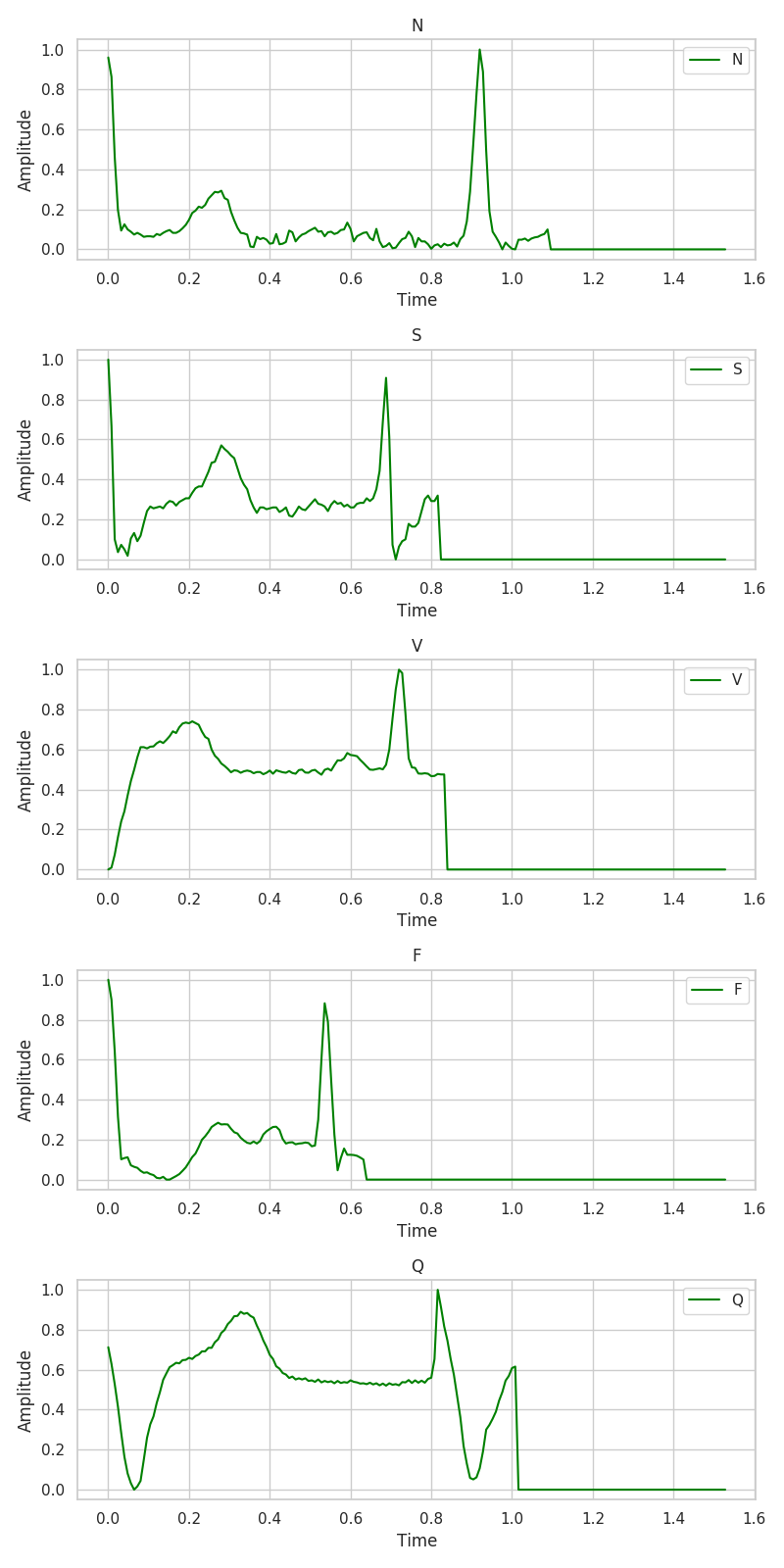
図1.3 クラス別ECG
それでは早速分類していきましょう。
2.CNN
- Pytorch: 1.1.0
- 12クラスのECG波形からの不整脈分類の研究[3]で用いられていた1d-CNNモデルを参考にします。
Dataset
- 検証セットは無し(訓練とテストのみ)。
- Data Augmentationは無し。
- Test Time Augmentationを用いる。
Code
# ---Hyperparameters---
num_tta = 5
ngpu = 1
device = torch.device("cuda:0" if (torch.cuda.is_available() and ngpu > 0) else "cpu")

# ---Transforms---
## If needed.

# --- Dataset---
class TrainECGDataset(Dataset):
    ### In order to inherit Dataset, define __len__ and __getitem__!

    def __init__(self, train_X, train_y, transforms=None):
        super().__init__()
        self.X = train_X
        self.y = train_y
        self.transforms = transforms

    def __len__(self):
      return len(self.X)

    def __getitem__(self, idx):
        sequence = self.X[idx]
        if self.transforms is not None:
            sequence = self.transforms(sequence)
        sequence = torch.unsqueeze(torch.from_numpy(sequence).float(), 0)
        target = torch.tensor(self.y[idx]).long()

        return sequence, target


class TestECGDataset(Dataset):
    ### Implement TTA (Test Time Augmentation).

    def __init__(self, test_X, test_y, transforms=None, tta=num_tta):
        super().__init__()
        self.X = test_X
        self.y = test_y
        self.transforms = transforms
        self.tta = tta

    def __len__(self):
        return len(self.X) * self.tta

    def __getitem__(self, idx):
        new_idx = idx % len(self.X)
        sequence = self.X[new_idx]
        if self.transforms is not None:
            sequence = self.transforms(sequence)
        sequence = torch.unsqueeze(torch.from_numpy(sequence).float(), 0)
        target = torch.tensor(self.y[new_idx]).long()

        return sequence, target

# ---DataLoader---
## If needed.
Model
- Residual connectionを組み込む(今回のネットワークは深くないので実際不要。)。
- Pre-activationとDropoutを用いる。
- Shortcut部分はダウンサンプリングのために、[1x1Conv1d, BatchNormalization, Max Pooling]を用いる。
Code
def weights_init(m):
    if isinstance(m, nn.Conv1d):
        nn.init.kaiming_normal_(m.weight)
        if m.bias is not None:
            nn.init.zeros_(m.bias)

class BaseBlock(nn.Module):

    def __init__(self, in_channels, out_channels):
        super(BaseBlock, self).__init__()
        self.deeppath = nn.Sequential(
                                      nn.BatchNorm1d(in_channels),
                                      nn.PReLU(),
                                      nn.Conv1d(in_channels, out_channels, kernel_size=4, stride=2, padding=1, bias=False),
                                      nn.BatchNorm1d(out_channels),
                                      nn.PReLU(),
                                      nn.Dropout(p=0.2, inplace=True),
                                      nn.Conv1d(out_channels, out_channels, kernel_size=3, stride=1, padding=1, bias=False)
                                     )
        self.shortcut = nn.Sequential(
                                      nn.Conv1d(in_channels, out_channels, kernel_size=1, stride=1, bias=False),
                                      nn.BatchNorm1d(out_channels),
                                      nn.MaxPool1d(kernel_size=2)
                                     )

    def forward(self, x):
      dp = self.deeppath(x)
      sc = self.shortcut(x)
      return dp + sc


class Flatten(nn.Module):

    def __init__(self):
        super(Flatten, self).__init__()

    def forward(self, x):
        return x.view(x.size(0), -1)


class ECGResNet(nn.Module):

    def __init__(self, block, num_classes=5):
        super(ECGResNet, self).__init__()
        self.net = nn.Sequential(
                                 nn.Conv1d(1, 16, kernel_size=4, stride=2, padding=1, bias=False),
                                 nn.BatchNorm1d(16),
                                 nn.PReLU(),
                                 nn.Conv1d(16, 64, kernel_size=4, stride=2, padding=1, bias=False),
                                 nn.BatchNorm1d(64),
                                 nn.PReLU(),
                                 nn.Dropout(p=0.2, inplace=True),
                                 nn.Conv1d(64, 64, kernel_size=3, stride=1, padding=1, bias=False),
                                 block(64, 128),
                                 nn.BatchNorm1d(128),
                                 nn.PReLU(),
                                 Flatten(),
                                 nn.Linear(128 * 24, num_classes)
                                )

    def forward(self, x):
        return self.net(x)


model = ECGResNet(BaseBlock).to(device)
model.apply(weights_init)
Training
- 今回はハイパーパラメータのチューニング等はしないので、検証データセットは作成せずに訓練させ、テストデータのF1スコアが最大になるようなモデルを求めます(K-Fold CVをする場合は訓練データのクラスが偏っているので、scikit-learnの
StratifiedKFoldなどを使って層別分割します(random_splitダメ、絶対))。 - loss:
CrossEntropyLoss - optimizer:
Adam - schedular:
ReduceLROnPlateau
Code
lr = 0.01
num_epochs = 4
batch_size=128

softmax = nn.Softmax()
criterion = nn.CrossEntropyLoss()
optimizer = Adam(model.parameters(), lr=lr)
schedular = ReduceLROnPlateau(optimizer, 'min', factor=0.1, patience=2, verbose=True)

train_losses = []
test_losses =[]
train_f1s = []
test_f1s = []

train_preds = []
test_preds = []

best_model_wts = copy.deepcopy(model.state_dict())
best_f1 = 0
best_probs = None
best_preds = None

datasets = {
    'train': TrainECGDataset(train_X, train_y),
    'test': TestECGDataset(test_X, test_y)
}


dataloaders = {
    'train': DataLoader(datasets['train'], batch_size=batch_size, shuffle=True),
    'test': DataLoader(datasets['test'], batch_size=batch_size, shuffle=False)
}

# ---Training and Evaluation---
start_time = time.time()

for epoch in range(num_epochs):
    print('Epoch {}/{}'.format(epoch, num_epochs - 1))
    print('-' * 20)

    for phase in ['test', 'train']:
        # 訓練無しでの性能を調べたいので先にテストセットの評価
        running_loss = 0 # of train or test
        epoch_loss = 0
        epoch_train_f1 = 0
        epoch_test_f1 = 0
        epoch_probs = None
        epoch_preds = None
        labels_list = None

        if phase == 'train':
            model.train()
        else:
            model.eval()

        for inputs, labels in dataloaders[phase]:
            inputs = inputs.to(device)
            labels = labels.to(device)
            optimizer.zero_grad()

            with torch.set_grad_enabled(phase == 'train'):
                outputs = model(inputs)
                loss = criterion(outputs, labels)
                if phase == 'train':
                    loss.backward()
                    optimizer.step()

            _, preds = torch.max(outputs, 1)
            probs = softmax(outputs).detach().cpu().numpy()
            preds = preds.detach().cpu().numpy()
            labels = labels.cpu().numpy()
            if epoch_probs is None:
                epoch_probs = probs
                epoch_preds = preds
                epoch_labels = labels
            else:
                epoch_probs = np.concatenate([epoch_probs, probs])
                epoch_preds = np.concatenate([epoch_preds, preds])
                epoch_labels = np.concatenate([epoch_labels, labels])

            running_loss += loss.item() * inputs.size(0)

        epoch_loss = running_loss / len(datasets[phase])

        if phase == 'train':
            schedular.step(epoch_test_f1)
            train_losses.append(epoch_loss)
            epoch_train_preds = epoch_preds
            train_preds.append(epoch_train_preds)
            epoch_train_f1 = f1_score(epoch_labels, epoch_train_preds, average='macro')
            train_f1s.append(epoch_train_f1)
            print('{} | Loss: {} | F1: {}'.format(phase, epoch_loss, epoch_train_f1))
        else:
            test_losses.append(epoch_loss)
            tta_probs = np.zeros((int(len(datasets[phase]) / num_tta), 5))
            for i in range(num_tta):
                tta_probs += epoch_probs[int(len(datasets[phase]) / num_tta) * i:int(len(datasets[phase]) / num_tta) * (i + 1)]
            tta_probs /= num_tta
            tta_preds = np.argmax(tta_probs, axis=1)
            test_preds.append(tta_preds)
            epoch_test_f1 = f1_score(test_y, tta_preds, average='macro')
            test_f1s.append(epoch_test_f1)
            print('{} | Loss: {} | F1: {}'.format(phase, epoch_loss, epoch_test_f1))

            if epoch_test_f1 > best_f1:
                best_f1 = epoch_test_f1
                best_probs = tta_probs
                best_preds = tta_preds
                best_model_wts = copy.deepcopy(model.state_dict())

time_elapsed  = time.time() - start_time
print('Training complete in {}m {}s.'.format(time_elapsed // 60, time_elapsed % 60))
print('Best f1: {}'.format(best_f1))

model.load_state_dict(best_model_wts)
Results
Code
#---Analysis---

## Loss and F1
fig = plt.figure(figsize=(10, 5))
ax1 = fig.add_subplot(121)
ax2 = fig.add_subplot(122)

ax1.plot(train_losses, label='train')
ax1.plot(test_losses, label='test')
ax2.plot(train_f1s, label='train')
ax2.plot(test_f1s, label='test')
ax1.set_xlabel("Epoch")
ax2.set_xlabel("Epoch")
ax1.set_ylabel("Loss")
ax2.set_ylabel("F1-score")
ax1.legend()
ax2.legend()
fig.tight_layout()
plt.savefig('loss_f1.png')

## Prediction
fig = plt.figure(figsize=(10, 8))
ax1 = fig.add_subplot(221)
ax2 = fig.add_subplot(222)
ax3 = fig.add_subplot(223)
ax4 = fig.add_subplot(224)

for i, ax in enumerate([ax1, ax2, ax3, ax4]):
    ax.plot(test_preds[i], label='pred')
    ax.plot(test_y, label='true')
    ax.set_xlabel('Data')
    ax.set_ylabel('Class')
    ax.set_title('Epoch: {}'.format(str(i)))
    ax.legend()
fig.tight_layout()
plt.savefig('test_classes.png')

## ROC
from sklearn.metrics import auc
classes = ['N', 'S', 'V', 'F', 'Q']

fig = plt.figure(figsize=(12, 8))
ax1 = fig.add_subplot(231)
ax2 = fig.add_subplot(232)
ax3 = fig.add_subplot(233)
ax4 = fig.add_subplot(234)
ax5 = fig.add_subplot(235)

for i, ax in enumerate([ax1, ax2, ax3, ax4, ax5]):
    fpr, tpr, _ = roc_curve(test_y_onehot[:, i], tta_probs[:, i])
    score = round(auc(fpr, tpr), 3)
    ax.plot(fpr, tpr, label='ROC curve (auc = {})'.format(score), color='red')
    ax.set_xlabel("False Positive Rate")
    ax.set_ylabel("True Positive Rate")
    ax.set_title(classes[i])
    ax.legend()
fig.tight_layout()
plt.savefig('roc.png')

## Confusion matrix
cm = confusion_matrix(test_y, tta_preds)
cm = cm / np.sum(test_y_onehot, axis=0).reshape(-1, 1)
df_cm = pd.DataFrame(cm, index=classes, columns=classes)
plt.figure(figsize = (6,5))
sns.heatmap(df_cm, cmap='Blues')
plt.show()
plt.savefig('confusion_matrix.png')
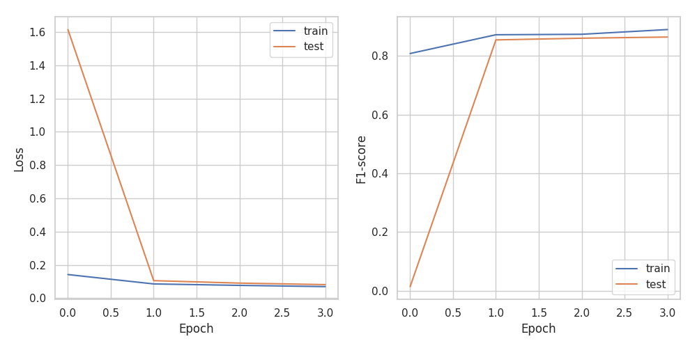
図2.1 損失とF値
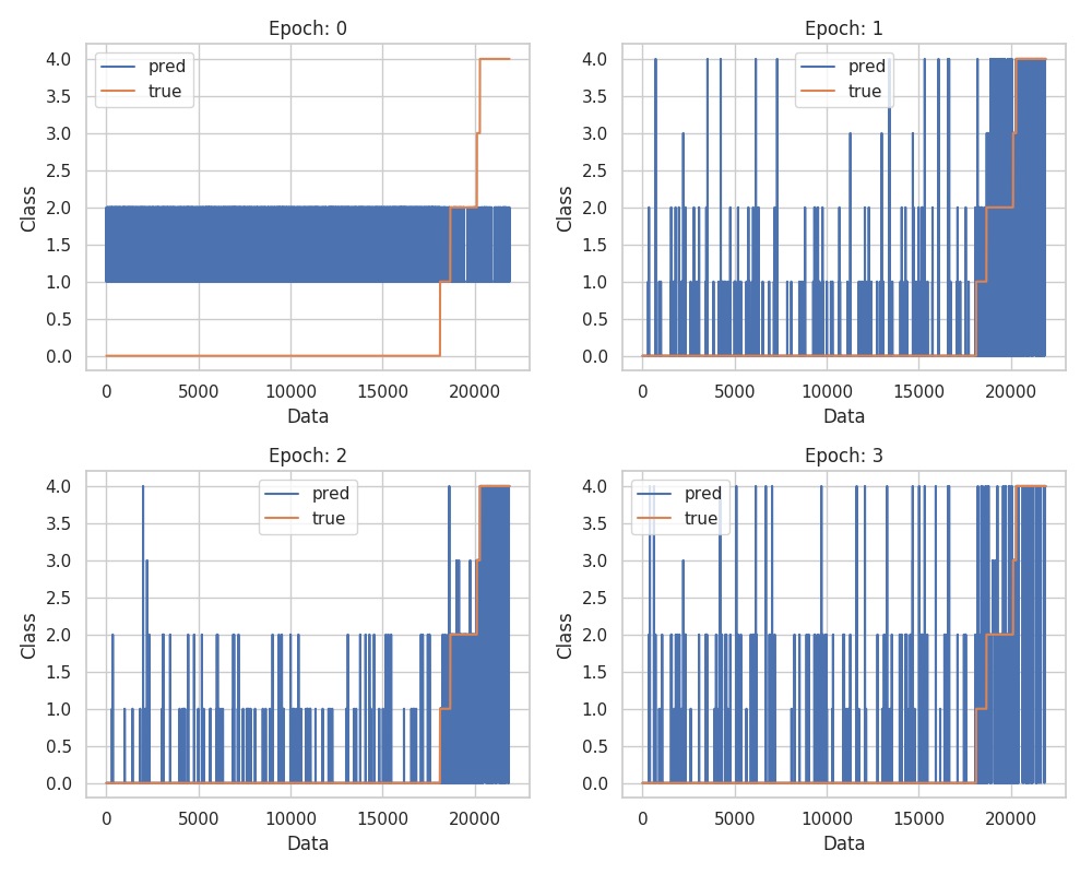
図2.2 予測クラスの推移 データごとの識別クラスの推移がなんとなく分かる。
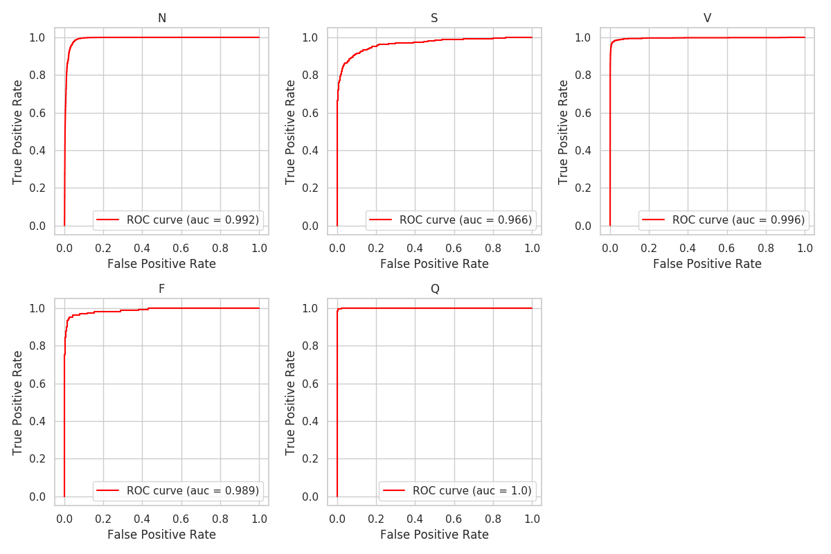
図2.3 ROC曲線
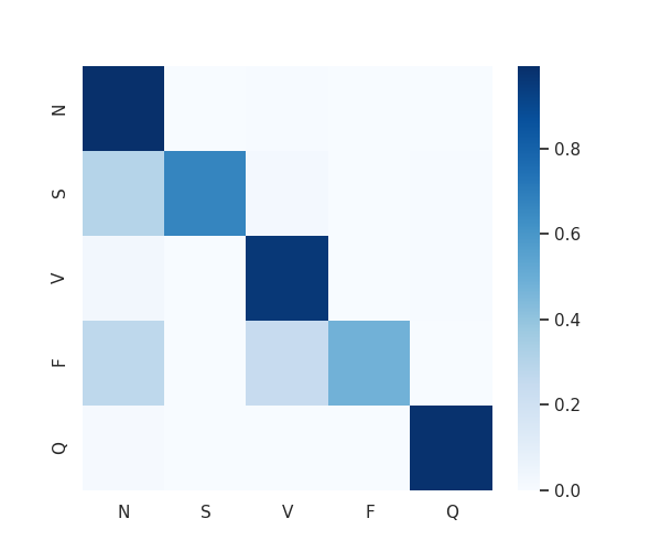
図2.4 混同行列のヒートマップ。縦軸が真のクラス、横軸が予測クラス。真のクラスのデータ数で正規化。SはN、FはVとNに誤識別している割合が多い。
3.コメント
精度よく分類できてることがわかります。[3]の研究での混同行列によると、機械学習でのECG分類の誤識別は実際の心臓専門医の誤識別と酷似しているようです。次回予定のモデル解釈でも触れる予定(未定)。
4.参考
[1] 病気が見えるvol.2循環器(書籍)
[2] "ECG Heartbeat Classification: A Deep Transferable Representation"(論文)
[3] "Cardiologist-level arrhythmia detection and classification in ambulatory electrocardiograms using a deep neural network"(論文)