【Python】初めての データ分析・機械学習（Kaggle）〜Part2〜

はじめに

今回取り組んだのは、Kaggleのチュートリアルである「Titanic」の問題です。

今日から初めて機械学習の勉強を始めたので、優秀な人のコードや記事をどんどん参考にしました笑

参照1：✔︎Introduction to Ensembling/Stacking in Python
Notebookで「Most voted」と評されていたコードです。(2020.3.10時点)

参照2:Pythonでアンサンブル(スタッキング)学習 & 機械学習チュートリアル in Kaggle

Introduction

今回取り組むタイタニック号のコンペの内容は、年齢、性別、同室者数、部屋のクラス、生死などの乗客に関するデータが与えられます。

そのデータを元に、
データの前処理
→データの可視化
→スタッキングモデル構築
→テストデータ
→評価

といった流れで、最後にはテストデータから構築したモデルを使って乗客の生死の予測をします。この予測がどれくらいあっているかもスコアの基準になります。

前回はデータの前処理・可視化を行いました！
前回の記事はこちら↓↓↓
【Python】初めての データ分析・機械学習（Kaggle）

本記事は、待ちに待ったスタッキングモデルの構築からです！！

では、早速スタッキングモデルの構築に取り掛かります！！

スタッキングアセンブルモデル

機械学習を今日から初めた私にとっては、そもそもスタッキング??アセンブル???わけわからん😭て感じです笑

そんな私でもこちらの記事を読んだら、なんとなく理解できました！
【機械学習】スタッキングのキホンを勉強したのでそのメモ

以下に簡単にまとめます。
あ、stackingは今回使うのでしっかり目に書きます笑

アセンブル学習

複数の学習器を組み合わせることで、予測エラーを小さくする手法。
(単一の学習器をそのまま使うのではない)

アセンブル学習の分類

1. voting

複数の学習器の平均や多数決をとる方法。

2. boosting

構成済みの学習器の誤りを反映して次段の弱学習器を形成する方法。

3. stacking

教師付き学習が前提。
初段の学習器の出力結果を次段の入力結果とする方法。
つまり初段と次段で２段会の学習を行います。

初段の学習

あらゆる学習器が用いられる（勾配ブースティング、ニューラルネット、ランダムフォレスト、K最近傍法など）。
Kaggleのコンペでは数このモデルから時には1000以上のモデルが組み合わされることもあるらしいです😳

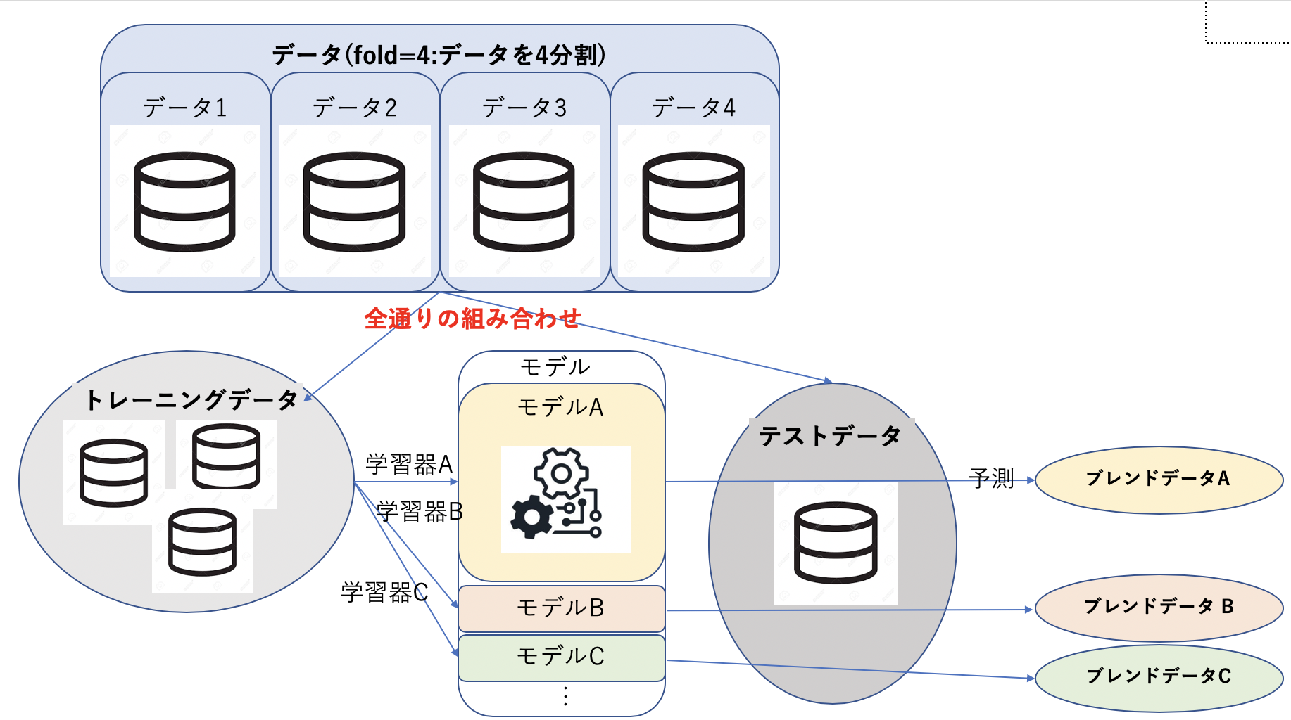
流れとしては以下の図のような感じで
1. データをトレーニング用とテスト用にわける（この時の分割数をfoldという）
2. トレーニング用データを用いて学習器で学習しモデルの構築
3. 構築したモデルをテストデータを用いて検証しブレンドデータを得る
4.1~3の工程を全てのデータの組み合わせ通り、全ての学習器で行う

次段の学習

正解データと初段の学習から得た全てのブレンドデータを使って、次段の学習の学習器を学習します。
1. 初段で得たブレンドデータを平均化する
2. 平均化されたブレンドデータを学習器に入力
3. 出力としてテストデータに対する予測結果を得る

モデルの作成

スタッキングアンサンブルモデルの理解が深まったところで、
早速、モデルを作成しましょう！

pythonで学習・予測するためのクラスの定義

class_define.py

#パラメータ
ntrain = train.shape[0] #891
ntest = test.shape[0] #418
SEED = 0
NFOLDS = 5 #5分割
kf = kFold(ntrain, n_folds = NFOLDS, random_state= SEED)

#Sklearn分類器を拡張
class SklearnHelper(object):
    def __init__(self, clf, seed=0, params=None):
        params['random_state'] = seed
        self.clf = clf(**params)

    def train(self, x_train, y_train):
        self.clf.fit(x_train, y_train)

    def predict(self, x):
        return self.clf.predict

    def fit(self, x, y):
        return self.clf.predict(x,y)

    def feature_importances(self,x,y):
        print(self.clf.fit(x,y).feature_importances_)

フォールド外予測(Out-of-Fold Prediction)

スタッキングでは、過学習を起こさないように交差検証を行います。

fold.py

def get_oof(clf, x_train, y_train, x_test):
    oof_train = np.zeros((ntrain,))
    oof_test = np.zeros((ntest,))
    oof_test_skf = np.empty((NFOLDS, ntest))

    for i, (train_index, test_index) in enumerate(kf): #NFOLDS回回す
       x_tr = x_train[train_index]
       y_tr = y_train[train_index]
       x_te = x_train[test_index]

       clf.train(x_tr, y_tr)

       oof_train[test_index] = clf.predict(x_te)
       oof_test_skf[i, :] = clf.predict(x_test)

    oof_test[:] = oof_test_skf.mean(axis=0)
    return oof_train.reshape(-1, 1), oof_test.reshape(-1,1)

初段の予測

今回は５つのモデルを使います。

1. RandomForestClassifier
2. AdaBoostClassifier
3. GradientBoostingClassifier
4. ExtraTreesClassifier
5. SVC

パラメータ

各モデルごとにパラメータをセットします。

• n_jobs:コア数。-1にすると全てのコア
• n_estimators:学習モデルの分類木の数。デフォルトは10。
• max_depth:気の最大深度。あまりに大きすぎるとオーバーフィットする。
• verbose:学習プロセス中にテキストを出力するか。0なら出力しない。3なら繰り返し出力する。

parameters.py

#Random Forest
rf_params = {
    'n_jobs':-1,
    'n_estimators':500,
    'warm_start':True,
    #'max_features':0.2,
    'max_depth':6,
    'min_samples_leaf':2,
    'max_features':'sqrt',
    'verbose':0
}

#Extra Trees
et_params = {
    'n_jobs':-1,
    'n_estimators':500,
    #'max_features':0.2
    'max_depth':8,
    'min_samples_leaf':2,
    'verbose':0
}

#AdaBoost
ada_params = {
     'n_estimators':500,
     'learning_rate':0.75
}

#Gradient Boosting
gb_params = {
    'n_estimators':500,
    #'max_features':0.2
    'max_depth':5,
    'min_samples_leaf':2,
    'verbose':0
}

さらに、Helpers via Python Classesで作成したクラスを用いて、５つの学習モデルのオブジェクトを作成します。

model_obj.py

rf = SklearnHelper(clf=RandomForestClassifier, seed=SEED, params=rf_params)
et = SklearnHelper(clf=ExtraTreesClassifier, seed=SEED, params=et_params)
ada = SklearnHelper(clf=AdaBoostClassifier, seed=SEED, params=ada_params)
gb = SklearnHelper(clf=GrandBoostingClassifier, seed=SEED, params=gb_params) 
svc = SklearnHelper(clf=SVC, seed=SEED, params=svc_params) 

ベースモデルへの入力データの準備

ベースモデルへの入力データをNumpy配列で準備します。

input_data.py

#入力データの作成
y_train = train['Survived'].ravel()
train = train.drop(['Survived'], axis=1)
x_train = train.values #学習データ
x_test = test.values #テストデータ

numpyのravel関数は初めて使ったので、こちらの記事を参照しました。
多次元の配列を1次元の配列で返すんですね！

５つのベースモデルで予測

学習データとテストデータを５つのベースモデルにおくり、交差検証(get_oof関数)を行い、予測します。

first_level_prediction.py

et_oof_train, et_oof_test = get_oof(et, x_train, y_train, x_test)#Extra Trees Classifier
rf_oof_train, rf_oof_test = get_oof(rf, x_train, y_train, x_test)#Random Forest Classifier
ada_oof_train, ada_oof_test = get_oof(ada, x_train, y_train, x_test)#AdaBoosting Classifier
gb_oof_train, gb_oof_test = get_oof(gb, x_train, y_train, x_test)#Gradient Boosting Classifier
svc_oof_train, svc_oof_test = get_oof(svc, x_train, y_train, x_test)#Support Vector Classifier

print("Rraining is complete!")

出力

Training is complete

特徴の重要度

予測に関わる特徴の重要度をみます。

feature_importances.py

rf_feature = rf.feature_importances(x_train, y_train)
et_feature = et.feature_importances(x_train, y_train)
ada_feature = ada.feature_importances(x_train, y_train)
gb_feature = gb.feature_importances(x_train, y_train)
svc_feature = svc.feature_importances(x_train, y_train)

出力

[ 0.12512537  0.20195675  0.03187994  0.02117736  0.0720603   0.02351993
  0.10877493  0.06461801  0.06974652  0.01355575  0.26758514]
[ 0.12082488  0.37460384  0.02701211  0.01713043  0.05593931  0.02854512
  0.04782111  0.08303969  0.04500919  0.02174382  0.1783305 ]
[ 0.028  0.012  0.02   0.062  0.04   0.01   0.69   0.014  0.05   0.004
  0.07 ]
[ 0.07626914  0.03373915  0.10207353  0.03738547  0.10223908  0.04940839
  0.39897827  0.01836958  0.07035654  0.02056481  0.09061604]

数値は
[Pclass Sex Age Parch Fare Embarked Name_length Has_Cabin FamilySize IsAlone Title]
に値する。
これらの乗客の特徴の重要度のリストを作成しデータフレームを作ります。

importanes_list.py

rf_features = [0.10474135,  0.21837029,  0.04432652,  0.02249159,  0.05432591,  0.02854371,
 0.07570305,  0.01088129 , 0.24247496,  0.13685733 , 0.06128402]
et_features = [ 0.12165657,  0.37098307  ,0.03129623 , 0.01591611 , 0.05525811 , 
 0.028157, 0.04589793 , 0.02030357 , 0.17289562 , 0.04853517,  0.08910063]
ada_features = [0.028, 0.008, 0.012, 0.05866667, 0.032 , 0.008,
 0.04666667, 0.001, 0.05733333, 0.73866667, 0.01066667]
gb_features = [0.06796144, 0.03889349, 0.07237845, 0.02628645, 0.11194395, 
 0.04778854, 0.05965792 , 0.02774745,  0.07462718,  0.4593142 ,  0.01340093]

特徴の重要度のデータフレームを作る

feature_importances.py

cols = train.columns.values
#特徴の重要度データフレームを作成
feature_dataframe = pd.DataFrame({'features': clos,
     'Random Forest feature importances': rf_features,
     'Extra Trees feature importances': et_features,
     'AdaBoosting feature importances': ada_features,
     'Gradient Boosting feature importances': gb_features
})

feature_dataframe

特徴の重要度データフレームのプロット

先ほど作った特徴の重要度のデータフレームをプロットします。

importances_df_plot.py

#Random Forest 散布図
trace = go.Scatter(
    y = feature_dataframe['Random Forest feature importances'].values,
    x = feature_dataframe['features'].values,
    mode = 'markers',
    marker = dict(
       sizemode = 'diameter',
       sizeref = 1,
       size = 25,
       color = feature_dataframe['Random Forest feature importances'].values,
       colorscale = 'Portland'
       showscale=True
    ),
    text = feature_dataframe['featture&'].values
)
data = [trace]

layout = go.Layout(
    autosize = True,
    title = 'Random Forest Feature Importance'
    hovermode = 'closest',
    yaxis = dict(
        title = 'Feature Importances',
        ticklen = 5,
        gridwidth = 2
    ),
    showlegend = False
)
fig = go.Figure(data=data, layout=layout)
py.iplot(fig, filename = 'scatter2010')


#Extra Trees 散布図
trace = go.scatter(
   y = featrue_dataframe['Extra Trees feature importances'].values,
   x = feature_dataframe['feature'],
   mode = 'markers',
   marker = dict(
       sizemode = 'diameter',
       sizeref = 1,
       size = 25,
       color = feature_dataframe['Extra Trees feature importances'].values,
       colorscale = 'Portland',
       showscale = True
   ),
   text = feature_dataframe['features'].values
)
data = [trace]

layout = go.Layout(
   autsize = True,
   title = 'Extra Trees Feature Importance',
   hovermode = 'closest',
   yaxis = dict(
      title = 'Feature Importance',
      ticklen = 5,
      gridwidth = 2
   ),
   showlegend = False
)
fig = go.Figure(data = data, layout = layout)
py.iplot(fig, filename = 'scatter2010')


# AdaBoost　散布図 
trace = go.Scatter(
    y = feature_dataframe['AdaBoost feature importances'].values,
    x = feature_dataframe['features'].values,
    mode='markers',
    marker=dict(
        sizemode = 'diameter',
        sizeref = 1,
        size = 25,

        color = feature_dataframe['AdaBoost feature importances'].values,
        colorscale='Portland',
        showscale=True
    ),
    text = feature_dataframe['features'].values
)
data = [trace]

layout= go.Layout(
    autosize= True,
    title= 'AdaBoost Feature Importance',
    hovermode= 'closest',

    yaxis=dict(
        title= 'Feature Importance',
        ticklen= 5,
        gridwidth= 2
    ),
    showlegend= False
)
fig = go.Figure(data=data, layout=layout)
py.iplot(fig,filename='scatter2010')

# Gradient Boosting　散布図 
trace = go.Scatter(
    y = feature_dataframe['Gradient Boost feature importances'].values,
    x = feature_dataframe['features'].values,
    mode='markers',
    marker=dict(
        sizemode = 'diameter',
        sizeref = 1,
        size = 25,
#       size= feature_dataframe['AdaBoost feature importances'].values,
        #color = np.random.randn(500), #set color equal to a variable
        color = feature_dataframe['Gradient Boost feature importances'].values,
        colorscale='Portland',
        showscale=True
    ),
    text = feature_dataframe['features'].values
)
data = [trace]

layout= go.Layout(
    autosize= True,
    title= 'Gradient Boosting Feature Importance',
    hovermode= 'closest',

    yaxis=dict(
        title= 'Feature Importance',
        ticklen= 5,
        gridwidth= 2
    ),
    showlegend= False
)
fig = go.Figure(data=data, layout=layout)
py.iplot(fig,filename='scatter2010')

plotlyでのプロットは初めてだったので、こちらの記事を参考にしました。

各特徴の重要度を平均化

feature_importance_mean.py

feature_dataframe['mean'] = feature_dataframe.mean(axis=1) #axis=1:行
feature_dataframe.head(3)

平均化した重要度をグラフにて可視化

importance_bar_graph.py

y = feature_dataframe['mean'].values
x = feature_dataframe['features'].values
data = [go.Bar(
            x= x,
             y= y,
            width = 0.5,
            marker=dict(
               color = feature_dataframe['mean'].values,
            colorscale='Portland',
            showscale=True,
            reversescale = False
            ),
            opacity=0.6
        )]

layout= go.Layout(
    autosize= True,
    title= 'Barplots of Mean Feature Importance',
    hovermode= 'closest',
#     xaxis= dict(
#         title= 'Pop',
#         ticklen= 5,
#         zeroline= False,
#         gridwidth= 2,
#     ),
    yaxis=dict(
        title= 'Feature Importance',
        ticklen= 5,
        gridwidth= 2
    ),
    showlegend= False
)
fig = go.Figure(data=data, layout=layout)
py.iplot(fig, filename='bar-direct-labels')

なるほど。このグラフを見る限りだと、「一人かどうか」「性別」「家族人数」が「生死」に特に大きく影響を与えているかもしれないのね。

これにて初段の学習は完了です！
続いては、次段の学習に取り組みます！

次段の予測

初段のベースモデルの予測値を使って、第二モデルを学習します！
まずは、ベースモデルの予測値のデータフレームの作成

first_model_output.py

base_predictions_train = pd.DataFrame({
     'Random Forest':rf_oof_train.ravel(),
     'Extra Trees':et_oof_train.ravel(),
     'AdaBoost':adaf_oof_train.ravel(),
     'GradientBoost':gb_oof_train.ravel()
     })
print('base_predictions_train.shape : ', base_predictions_train.shape)
base_predictions_train.head(5)

出力

base_predictions_train.shape : (891, 4)

ベースモデルの予測値の相関

predictions_cor.py

data = [go.Heatmap(
    z = base_predictions_train.astype(float).corr().values,
    y = base_predictions_train.columns.values,
    x = base_predictions_train.columns.values,
    colorscale = 'Viridis',
    showscale = True,
    reversescale = True
    )
]
py.iplot(data = data, filename = 'labelled_heatmap')

第二モデルの学習データとテストデータを作成

ベースモデルの予測値を結合して、第二モデルの学習データとテストデータを作成します！

data_making.py

x_train = np.concatenate((et_oof_train, rf_oof_train, ada_oof_train, gb_oof_train, svc_oof_train ), axis = 1)
x_test = np.concatenate((et_oof_test, rf_oof_test, ada_oof_test, gb_oof_test, svc_oof_test ), axis = 1)
print('x_train.shape: ', x_train.shape)
print('x_test.shape: ', x_test.shape)

出力

x_train.shape: (891, 5)
x_test.shape: (418, 5)

これで、第二モデル用の学習データとテストデータの準備ができました！

XGBoostで第二モデルの学習

第二モデルにはXGBoostを使用します。

XGBoost.py

gbm = xgb.XGBClassofier(
    #learing_rate = 0.02,
  n_estimators = 2000,
  max_depth = 4,
  min_child_weight = 2,
  gamma = 0.9,
  subsample = 0.8,
  colsample_bytree = 0.8,
  objective = 0.8,
  nthread = -1,
  scale_pos_weight = 1
  ).fit(x_train, y_train)
predictions = gbm.predict(x_test)

パラメータ

• max_depth:木の最大深度。あまりに大きくすると過学習となる。
• gamma:最適化パラメータ。大きくすると控えめなアルゴリズムになる。
• eta:過学習を防止するためのパラメータ。

Kaggle提出用のcsvファイルの書き出し

submission_kaggle.py

StackingSubmission = pd.DataFrame({'PassengerId': PassengerId, 'Survived': predictions})
StackingSubmission.to_csv("StackingSubmission.csv", index = False)

まとめ

Kaggleのチュートリアルの「タイタニック号」の問題を、アンサンブル（スタッキング）学習で取り組んでみました！

本記事はモデル構築についてから書きました。
流れとしては、

1. 第１段階の学習

   • データを学習用とテスト用に分割
   • 使用する各モデルで学習
   • 学習後テストデータで予測
   • 各モデルで特徴の「重み」の算出
   • 特徴の「重み」を全モデルで平均化

2. 第2段階の学習

   • ベースモデルの予測値を使って第二段階モデルを学習

機械学習を用いた簡単な予測ができるようになって大変満足です笑
どんどんこれからkaggleに取り組み、アウトプットを続けていきたいと思います！

最後まで本記事を見てくださり、ありがとうございました！！