はじめに
Julia言語で、数値データを手っ取り早くグラフとかに可視化するならば現状
Plots Makieの2択が有力ではないでしょうか。
今回はそのうちPlotsを使ってみます
Plotsって?
特徴として
・複数のバックエンドを、ほぼ単一の記述で扱うことができる
が上げられ、様々な特徴の可視化パッケージを、それぞれ個別に関数・記法を覚えていては無駄が多いので
フロントエンド としてPlotsで仕様を吸収し それら使用を気にすることなくバックエンドを扱う事ができます。
詳細は、docs.juliaplots.orgに詳しいです。
(以下の内容はほとんど、docsの内容となります。)
バックエンド
扱える可視化パッケージ
それぞれ別個であるエンジンのJulia Wrapperのようです。
| バックエンド名 | 説明 |
|---|---|
GR |
デフォルト・軽い |
Plotly/PlotlyJS
|
キレイ・インタラクティブ(ブラウザ表示) |
PyPlot |
キレイ・インタラクティブ、PyCallを使ったMatplotlib |
| PGFPlotsX | Texによるグラフ生成(pkg以外に必要条件が多数あり未確認です・・) |
InspecterDR |
軽い、2D限定 |
UnicodePlots |
REPL上でCUI表示、そりゃ軽い |
HDF5 |
表示ではなく、「.hdf5」形式で可視化データをファイル操作する |
私は普段GR、見た目キレイでPyPlotか、3DでグリグリでPlotlyといったところです。
準備
まだPlotsパッケージをいれてないなら、パッケージモードで
pkg>add Plots
#さらにGRを除く他のバックエンドが必要なら、 例:PyPlot
pkg>add PyPlot
と入れておきましょう
(pkgにより、更に追加のインストールがいる場合もあります。)
使用例
動作確認
using Plots
gr()           #バックエンドの指定・切り替え(デフォはGRなので、なくてもよい)
plot(sin)      #関数sinをプロット。 plot(関数;初期値,終了値)で初期値・終了値を省略したもの

とsin関数が表示されるはずです。(REPLからなら別窓)
以下、特に指定ないものはバックエンドgr()でJupyter notebook出力です。
プロットに追加
plot(sin)
plot!(cos)  #関数cosを追加。 plot!((ベースのプロット,) 追加関数,...) ,ベース関数の省略時は直前のプロット

追加は何度も重ねられます。
p=plot(...)で変数に残しておけば直前のもでなくてもplot!(p,関数,...)で可能です。
また、current()で直前プロットを拾う事もできます。
プロット内表示の調整
plot(x->(x^2-1),               #無名関数による x²-1
    xlabel       ="X_value",   #X軸のラベル
    ylabel       ="Y_value",   #Y軸のラベル
    label        ="LABEL",     #凡例のテキスト
    xlims        =(-3,3),      #X軸の範囲
    ylims        =(-3,3),      #Y軸の範囲
    aspect_ratio =0.5,         #表示のY/Xのアスペクト比
    title        ="TITLE",     #タイトル
    linecolor    =:blue,       #線の色
    linewidth    =5,           #線幅
    linestyle    =:dot,        #線種
    size         =(400,300),   #プロットのサイズ
)

プロットの調整のごく一部ですが、更にAlias等も沢山あります。
詳細は先ほどのdocsのAttributesやsupported Attributes(対応/未対応)をちょくちょく確認しましょう。
毎回 同じような設定の場合は最初のバックエンド切替えでgr(設定)やdefault(設定)で宣言しておけば、手間が省けます。
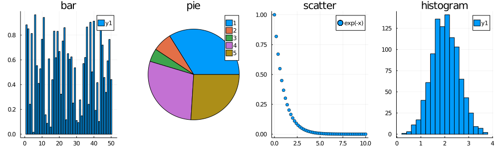
グラフの種類
入力するデータタイプにもよりますが、seriestypeの指定でグラフの種類を変更できます。
#plot(データ配列,st=:グラフの種類,...) stはseriestypeのAlias
p1=plot(rand(50),st=:bar,title="bar")                           #棒グラフ
p2=plot(rand(5),st=:pie,title="pie")                            #円グラフ
x=0:0.2:10
p3=plot(x,exp.(-x),st=:scatter,title="scatter",label="exp(-x)") #散布図 plot(xデータ,yデータ,st=...)
p4=plot(rand(1000)+rand(1000)+rand(1000)+rand(1000),
        st=:histogram,title="histogram")                        #ヒストグラム(4回乱数を足したデータを自動処理)
plot(p1,p2,p3,p4,layout=(1,4),size=(1000,300))                  #上記プロットを一気に1×4レイアウトでプロット
docsによると
:none,:line,:path,:steppre,:steppost,:sticks,:scatter,:heatmap,:hexbin,:barbins,:barhist,:histogram,:scatterbins,:scatterhist,:stepbins,:stephist,:bins2d,:histogram2d,:histogram3d,:density,:bar,:hline,:vline,:contour,:pie,:shape,:image,:path3d,:scatter3d,:surface,:wireframe,:contour3d,:volume
と種類があるようです。
この辺りのいくつかはst=で指定しなくても、そのままの関数が用意されており
#データ作成
x=-3:0.2:3
y=x
z=@. exp(-(x^2+y'^2))                                    #z=exp(-(x²+y²)) , yの[']転置と@.マクロに注意
#各プロット
p1=heatmap(z,title="heatmap")                            #ヒートマップ heatmap(2次元データ,...)
p2=contour(x,y,z,title="contour")                        #コンター図   contour(xデータ,y,z,...)
p3=wireframe(x,y,z,title="wireframe")                    #3Dのワイヤーフレーム表記
p4=surface(x,y,z,title="surface")                        #3Dの曲面表示
plot(p1,p2,p3,p4,layout=(1,4),size=(1500,250),fmt=:png)  #1×4表記 (少し重たくなるので、後述のフォーマットpng)
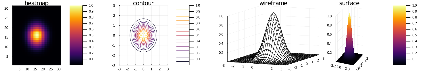
とプロットできます。
上記のデータ入力は一例で、複素数データを2D極座標で表示してくれたりなど柔軟さがあります。
これもdocsのInput Dataを確認するとよいでしょう。
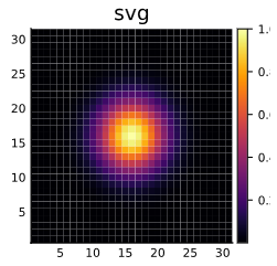
出力形式(pngとsvg)
先ほどのplotでfmt=:png を指定しましたが、デフォルでは:svg形式で出力されます。
:pngは画像形式ですが、:svgは座標等の描画情報を持っており、wireframeプロット等したとき
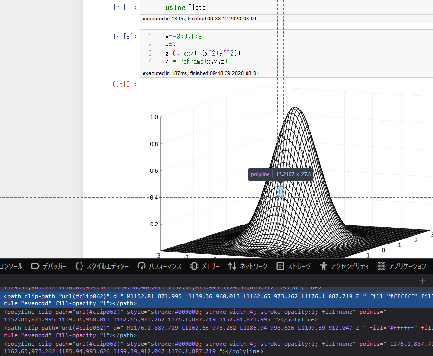
の様に、Jupyterではブラウザが頑張って線を引き、動作が重たくなってしまう場合があります。
また、大概の例で:svgの方が表示はキレイなのですが、PyPlotバックエンドのheatmapで
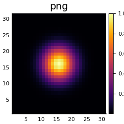
の様に妙な線が入ってしまう場合があるので、場合によって使い分けるといいと思います。
カラースキーム
レンジ色のカラースキームを調整します。
seriescolorを指定しますが、細かくはpalette cgrad関数で指定します。
#plot(データ配列,c=:カラースキームの種類,...) colorはseriescolorのAlias(他にc等)
x=y=range(-10,10,length=51)
r(x,y)=sqrt(x^2+y^2+0.0)+1e-10
z(x,y)=sin(r(x,y))/r(x,y)

p1=surface(x,y,z.(x,y'),color=palette(:ice    ,10) ,title="palette(:ice,10)")     #パレットに:ice指定(2番目の引数は分割数)
p2=surface(x,y,z.(x,y'),color=palette(:thermal,10) ,title="palette(:thermal,10)") #パレットに:thermal指定
p3=surface(x,y,z.(x,y'),color=cgrad(:thermal)      ,title="cgrad(:thermal)")      #グラデーションで:thermal指定
p4=surface(x,y,z.(x,y'),color=:thermal             ,title=":thermal")             #省略表記は上記グラデーション

plot(p1,p2,p3,p4,layout=(2,2),size=(1500,600))
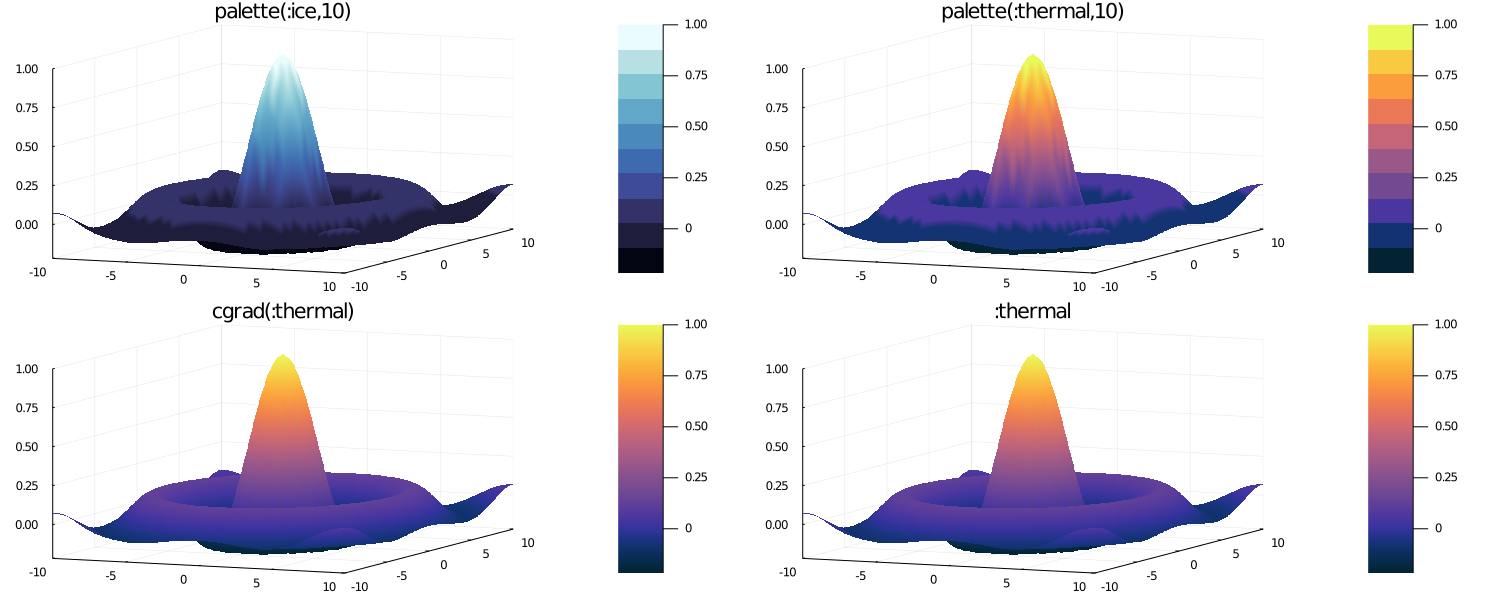
余り代り映えしていませんが、カラースキームが変更されています。
他に:rainbow :blues :Spectralなど、docsのcolorschemesで確認できます。
また、上記のpalette cgrad関数は自分で色を指定して(RGB可)、単体で出力確認もできます。
palette([:red,:white,:purple],15 ,rev=true) |>display   # rev=trueは反転
cgrad([RGB(255/255,0,0),:lightgreen])       |>display   # RGB関数は各色0~1範囲
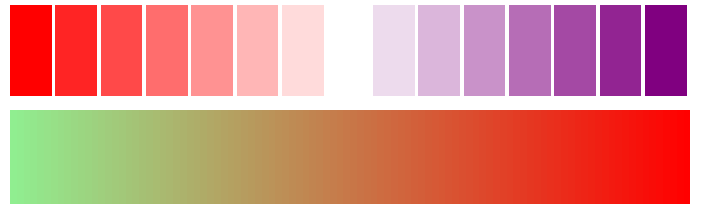
線色等でも使ってましたが、X11の色名称(Wikipedia)をサポートしている様で、なんとなく入れて作りたいものが大体できるでしょう。
動画の出力
出力したプロットをpng形式でtmpフォルダに保存し、ffmpegに投げるようです。
その為Juliaとは別にffmpegのインストールとPATHを通しておく必要があります。
(古いverの認識でした。現在は自動で入るようです。コメント欄参照、感謝)
gif動画の生成
anim = @animate for i in 0:0.1:2            #@animateマクロでfor文内ループ毎をフレームとしたpngファイル生成
    x=0:0.1:2
    y1=@. sin(pi*(x+i))
    y2=@. cos(pi*(x+i))
    plot(x,y1,label="sin(π(x+$i))",size=(250,250))   #ラベルのテキストに$(変数)を使う事でラベル表示も変化
    plot!(x,y2,label="cos(π(x+$i))")                 #最後のプロットがpngとして格納される
end                                                  #endの後にever 5 等とすると5フレーム毎に残す
gif(anim,fps=30,"sin_cos.gif")                       #gif出力,fpsとファイル名指定はオプション(tmp.gifがデフォ)
gif()以外にも他にもmp4(),mov(),webm()あるようです。
動画生成は長めに作ると完成まで時間がかかり、確認が遅くなるのですがJupyter notebookでの動画に限り
・JuliaのJupyterでプロット動画を素早く確認する#折衷案
を利用すると、各フレームをプロット出力しながらの確認にすることができます。
機能さがし(追記)
docsを見るのが一番ですが
plotattr(:Plot)
plotattr(:Series)
plotattr(:Subplot)
plotattr(:Axis)
とすることで、それぞれのattributes一覧が出力されます
Defined Plot attributes are:
background_color, background_color_outside, display_type, dpi, extra_kwargs, extra_plot_kwargs, fontfamily, foreground_color, html_output_format, inset_subplots, layout, link, overwrite_figure, plot_title, plot_title_location, plot_titlefontcolor, plot_titlefontfamily, plot_titlefonthalign, plot_titlefontrotation, plot_titlefontsize, plot_titlefontvalign, pos, show, size, tex_output_standalone, thickness_scaling, warn_on_unsupported, window_title
Defined Series attributes are:
arrow, bar_edges, bar_position, bar_width, bins, colorbar_entry, connections, contour_labels, contours, extra_kwargs, fill_z, fillalpha, fillcolor, fillrange, group, hover, label, levels, line_z, linealpha, linecolor, linestyle, linewidth, marker_z, markeralpha, markercolor, markershape, markersize, markerstrokealpha, markerstrokecolor, markerstrokestyle, markerstrokewidth, normalize, orientation, primary, quiver, ribbon, series_annotations, seriesalpha, seriescolor, seriestype, show_empty_bins, smooth, stride, subplot, weights, x, xerror, y, yerror, z, zerror
Defined Subplot attributes are:
annotations, aspect_ratio, background_color_inside, background_color_legend, background_color_subplot, bottom_margin, camera, clims, color_palette, colorbar, colorbar_fontfamily, colorbar_title, colorbar_title_location, colorbar_titlefontcolor, colorbar_titlefontfamily, colorbar_titlefonthalign, colorbar_titlefontrotation, colorbar_titlefontsize, colorbar_titlefontvalign, extra_kwargs, fontfamily_subplot, foreground_color_legend, foreground_color_subplot, foreground_color_title, framestyle, left_margin, legend, legendfontcolor, legendfontfamily, legendfonthalign, legendfontrotation, legendfontsize, legendfontvalign, legendtitle, legendtitlefontcolor, legendtitlefontfamily, legendtitlefonthalign, legendtitlefontrotation, legendtitlefontsize, legendtitlefontvalign, margin, projection, right_margin, subplot_index, title, titlefontcolor, titlefontfamily, titlefonthalign, titlefontrotation, titlefontsize, titlefontvalign, titlelocation, top_margin
Defined Axis attributes are:
discrete_values, draw_arrow, flip, foreground_color_axis, foreground_color_border, foreground_color_grid, foreground_color_guide, foreground_color_minor_grid, foreground_color_text, formatter, grid, gridalpha, gridlinewidth, gridstyle, guide, guide_position, guidefontcolor, guidefontfamily, guidefonthalign, guidefontrotation, guidefontsize, guidefontvalign, lims, link, minorgrid, minorgridalpha, minorgridlinewidth, minorgridstyle, minorticks, mirror, rotation, scale, showaxis, tick_direction, tickfontcolor, tickfontfamily, tickfonthalign, tickfontrotation, tickfontsize, tickfontvalign, ticks, widen
aliasではないので、機能名前っぽいはずです。
ここから欲しい感じのを探して更に
plotattr("camera")
camera {NTuple{2, Real}}
cam, cameras, view_angle, viewangle

Sets the view angle (azimuthal, elevation) for 3D plots
Subplot attribute,  default: (30, 30)
と docsと同様の内容ですが、aliasと機能が分かるで当たりをつけて探しやすくなると思います。
(他にいい方法があるなら教えてほしい)
その他
時間短縮
表示までが遅いと思った人もいるかもしれません。
Plotsは巨大パッケージで、初回のJITコンパイルが結構長めです。対策としては、PackageCompilerをもちいるのが有力で
・PackageCompiler.jlでPlotsの呼び出しを高速化する2020年7月版
が参考になります。
(オプションで、更にprecompileする関数の指定も可能なのですが、やりすぎると表示されない謎動作等が多発します・・・)
また現在(2020年8月)はJuliaの安定版はver1.5.0で、これまでも高速化されてきましたが
・Nightly builds1.6.0-devでは大幅に高速化
といった情報もあるので期待 and 試してみるとよいと思います。
(2021年4月)1.6.0安定版でましたね。1.5.0の頃から2倍近く早くなってんじゃないでしょうか
Juliaは最新版で結構安定しているので、随時更新すると良いと思います。
機能しない等エラーについて(2021年08月追記)
Plotsまわりは複雑で上手く機能が動かない事もあるのですが、デフォルトのバックエンドGR要因が多々あるようです。
下記コメント欄、プロットサイズがおかしい問題などはGRversionが古い場合がある様なのでパッケージモードで
pkg> up GRで解決するかもしれません。
また、別のバックエンド指定(特にPyPlot)ではちゃんと機能したりする場合、GRは諦めた方が早いかもしれません。