動作環境
Xeon E5-2620 v4 (8コア) x 2
32GB RAM
GeForce GT 730 1GB GDDR5
CentOS 6.9 (64bit)
NCAR Command Language Version 6.3.0
for WRF3.7.1, WPS3.7.1
  openmpi-1.8.x86_64 とその-devel
  mpich.x86_64 3.1-5.el6とその-devel
  gcc version 4.4.7 (とgfortran)
for WRF3.9, WPS3.9
  Open MPI v2.1.1
  gcc version 4.9.2 (とgfortran; devtoolset-3使用)
 NetCDF v4.4.1.1, NetCDF (Fortran API) v4.4.4
Python 2.6.6 (r266:84292, Aug 18 2016, 15:13:37)
Python 3.6.0 on virtualenv
GNU bash, version 4.1.2(2)-release (x86_64-redhat-linux-gnu)
date (GNU coreutils) 8.4
tmux 1.6-3.el6
WRF(Weather Research and Forecasting Model)とその前処理であるWPS関連。
v0.1: WPS > NCL > wps_plot_geo_em_with_marker_180511.ncl > v0.1 > geo_em.d01.ncデータの地図上表示 + markerの表示
処理概要
WPSで生成される以下のファイルがある (ネスト設定で生成)。
- geo_em.d01.nc
- geo_em.d02.nc
- geo_em.d03.nc
これらの緯度経度関係を確認したい。
参考
-
https://www.ncl.ucar.edu/Support/talk_archives/2012/0417.html
- 緯度経度はXLONG_UとXLAT_Uを使う
-
NCL > array > 2つのarrayを足す > array_append_record
- d02とd03のarrayの合成
code v0.2
wps_plot_geo_em_with_marker_180511.ncl
load "$NCARG_ROOT/lib/ncarg/nclscripts/csm/gsn_code.ncl"
load "$NCARG_ROOT/lib/ncarg/nclscripts/wrf/WRFUserARW.ncl"

;
; v0.2 May. 11, 2018
;   - overlay markers of [d02] and [d03] instead of constant latitude, longitude
; v0.1 May. 11, 2018
;   - overlay markers defined with xs[], ys[]
;   - plot [geo_em.d01.nc] file
;

begin

  infile_d01 = addfile("./geo_em.d01.nc","r")
  infile_d02 = addfile("./geo_em.d02.nc","r")
  infile_d03 = addfile("./geo_em.d03.nc","r")

  type = "x11"

; 1. get range of d02
  lats = infile_d02->XLAT_U(0,:,:)
  lons = infile_d02->XLONG_U(0,:,:)
  lat_min_d02 = min(lats)
  lat_max_d02 = max(lats)
  lon_min_d02 = min(lons)
  lon_max_d02 = max(lons)

; 2. get range of d03
  lats = infile_d03->XLAT_U(0,:,:)
  lons = infile_d03->XLONG_U(0,:,:)
  lat_min_d03 = min(lats)
  lat_max_d03 = max(lats)
  lon_min_d03 = min(lons)
  lon_max_d03 = max(lons)

; 3. plot WPS output
  wks = gsn_open_wks(type,"plt_geo_4")

  opts = True
  opts@MainTitle = "GEOGRID FIELDS"

  ter = infile_d01->HGT_M(0,:,:)

  res = opts
  res@cnFillOn = True

  contour = wrf_contour(infile_d01,wks,ter,res)

  pltres = True
  pltres@PanelPlot = True  ; to overlay marker
  mpres = True
  plot = wrf_map_overlays(infile_d01,wks,(/contour/),pltres,mpres)

; 4. add markers
  gsres = True ; set some resource
  gsres@gsMarkerSizeF = 10.
  gsres@gsMarkerIndex = 16.  ; filled circles
  gsres@gsMarkerColor = 0  ; white
  xs_d02 = (/lon_min_d02,lon_max_d02,lon_max_d02,lon_min_d02/)
  ys_d02 = (/lat_min_d02,lat_min_d02,lat_max_d02,lat_max_d02/)
  xs_d03 = (/lon_min_d03,lon_max_d03,lon_max_d03,lon_min_d03/)
  ys_d03 = (/lat_min_d03,lat_min_d03,lat_max_d03,lat_max_d03/)
  xs = array_append_record(xs_d02, xs_d03, 0)
  ys = array_append_record(ys_d02, ys_d03, 0)
  plot1 = gsn_add_polymarker(wks,plot,xs,ys,gsres)

  draw(plot)
  frame(wks)

end
実行例
日本近海のデータでは以下のように表示される。
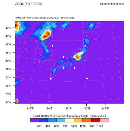
d02とd03は白丸markerでの表示。
ネストの位置関係が把握できるようになった。