GOSのサンプリング地点をRで可視化する

概要

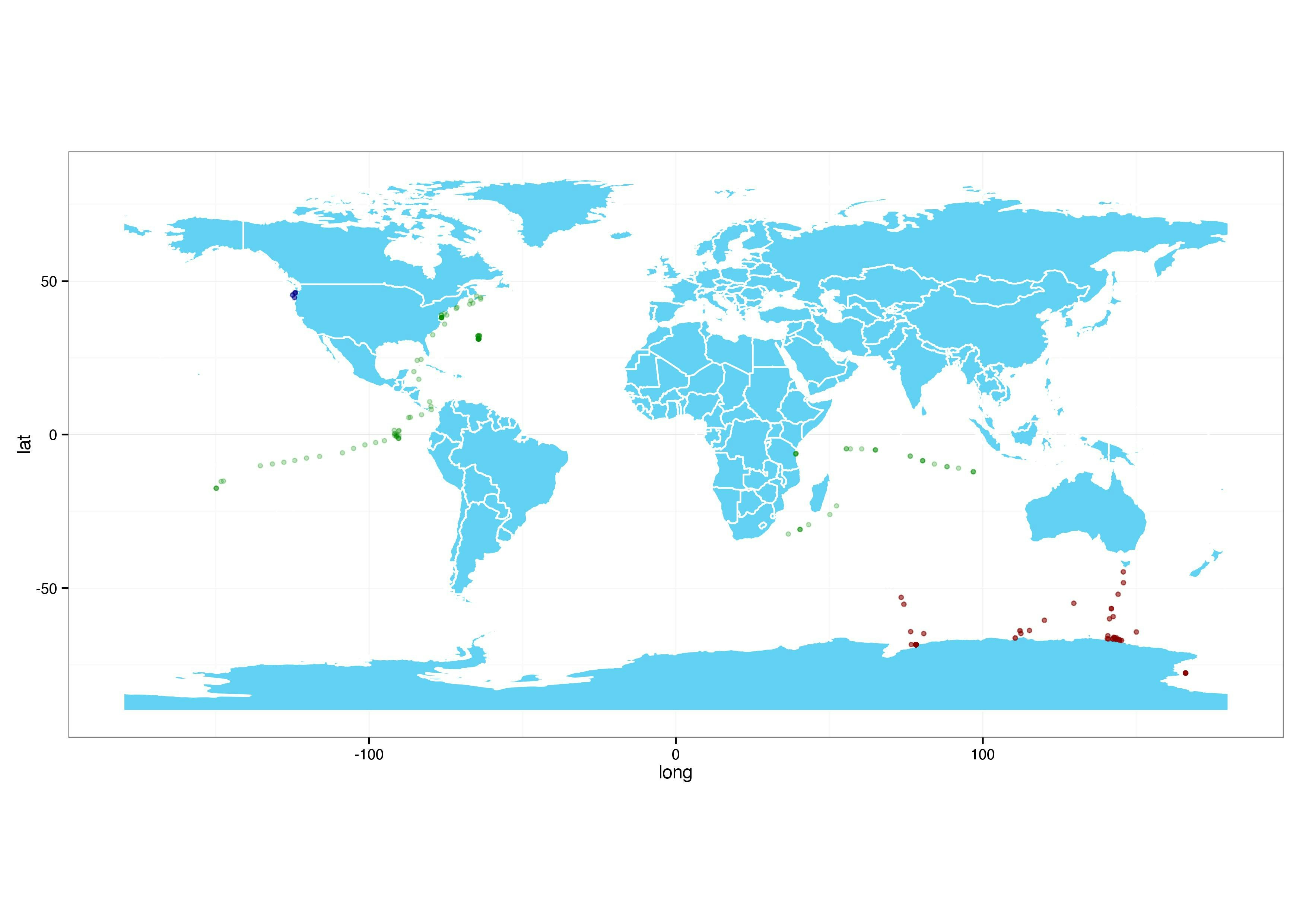
あるプロジェクトにおけるサンプルのサンプリングポイントがどこだかを可視化しました．
（ただし，メタデータの全てを得られたわけではないので，ここにあるのが全てというわけではありません）

Rで描く

# install.packages("maptools")
# install.packages("rgeos")
# install.packages("gpclib")

rm(list=ls())

library(maptools) 
library(rgeos)
library(ggplot2) 
gpclibPermit() 
theme_set(theme_bw()) 


world.shp <- readShapeSpatial("~/Downloads/TM_WORLD_BORDERS-0/TM_WORLD_BORDERS-0.3.shp") 

# check for region-id - Use "FIPS" 
head(world.shp@data) 

## see licence, not GPL 
# world.shp.p <- fortify.SpatialPolygonsDataFrame(world.shp, region="FIPS") 
world.shp.p <- fortify(world.shp, region="FIPS") 

world <- merge(world.shp.p, world.shp, by.x="id", by.y="FIPS") 

head(world) 
dim(world) 

# only the worldmap 
p <- ggplot(data=world, aes(x=long, y=lat, group=group)) + 
geom_polygon(fill="#63D1F4") 
p <- p + geom_path(color="white") + coord_equal() 
plot(p)
ggsave(p, width=11.69, height=8.27, file="world_map.jpg") 

## Add some locations 
d <- read.table("~/Desktop/gcos_point.txt", header=T)
colnames(d) <- c("lat", "long")

dat <- read.table("~/Downloads/CAM_PROJ_GOS.csv", header=T, sep=",")
colnames(dat)[grep("LATITUDE", colnames(dat))] <- "lat"
colnames(dat)[grep("LONGITUDE", colnames(dat))] <- "long"



p1 <- p + geom_point(data = dat, aes(group = NULL), shape=20, 
                      color="#00880040") 
ggsave(p1, width=11.69, height=8.27, file="world_map_2.jpg") 




dat2 <- read.table("~/Downloads/CAM_PROJ_AntarcticaAquatic.csv", header=T, sep=",")
colnames(dat2)[grep("LATITUDE", colnames(dat2))] <- "lat"
colnames(dat2)[grep("LONGITUDE", colnames(dat2))] <- "long"
p2 <- p1 + geom_point(data = dat2, aes(group = NULL), shape=20, 
                      color="#88000040") 
ggsave(p2, width=11.69, height=8.27, file="world_map_3.jpg") 



dat3 <- read.table("~/Downloads/CAM_P_0001024.csv", header=T, sep=",")
colnames(dat3)[grep("LATITUDE", colnames(dat3))] <- "lat"
colnames(dat3)[grep("LONGITUDE", colnames(dat3))] <- "long"
p3 <- p2 + geom_point(data = dat3, aes(group = NULL), shape=20, 
                      color="#00008840") 
ggsave(p3, width=11.69, height=8.27, file="world_map_4.jpg") 

サンプリングポイントが重なっている部分は濃くなっています．

参考

• http://r.789695.n4.nabble.com/Projecting-data-on-a-world-map-using-long-lat-td3081298.html
• http://jeffreybreen.wordpress.com/tag/raster/
• 世界地図のshapeデータ: http://thematicmapping.org/downloads/world_borders.php
• プロジェクトについて: http://www.jcvi.org/cms/research/projects/gos/overview/
• プロジェクトのメタデータ: http://camera.calit2.net