概要
すぐに使えるKNBCコーパスを対象に、モダンなRの書き方でテキスト解析したときのメモです。TF-IDFや共起頻度(ネットワーク作成)、LDAやGloVeまでをパッケージで実行しました。
定義・設定
最初に処理で利用するライブラリの読み込みや定数・関数の定義。
library(pacman)
library(widyr)

# 読み込むパッケージ
SET_LOAD_PACKAGE <- c("tidyverse", "Rcpp", "chunked", "tidytext", "visNetwork", "textmineR", "Matrix", "topicmodels", "LDAvis", "text2vec")

# コーパスファイルの設定
SET_CORPUS_FILE <- list(
  DOWNLOAD_URL = "http://nlp.ist.i.kyoto-u.ac.jp/kuntt/KNBC_v1.0_090925.tar.bz2",
  DIST_FILE = "KNBC.tar.bz2"
)
SET_TARGET_DIR <- list(
  EXTRACT_DIR = "knbc_corpus",
  READ_DIR = "knbc_corpus/KNBC_v1.0_090925/corpus2/"
)
SET_STAGING_FILE = "knbc.csv"

# ストップワード設定
SET_STOP_WORD <- c("こと", "もの", "私", "よう", "これ", "の")
# MeCabの{Rcpp}ラッパー定義
Sys.setenv("PKG_LIBS" = "-lmecab")
callCppMeCab <- Rcpp::cppFunction(
  code = 'DataFrame callCppMeCab(SEXP str) {
  std::string input = Rcpp::as<std::string>(str);
  std::vector<std::string> surface, feature;

  // MeCabタガーを生成して、入力文の形態素解析結果を受け取る
  MeCab::Tagger *tagger = MeCab::createTagger("-l 2");
  const MeCab::Node* node = tagger->parseToNode(input.c_str());

  std::vector<std::string> strs;
  for (; node; node = node->next) {
    if (node->stat == MECAB_NOR_NODE || node->stat == MECAB_UNK_NODE) {
      surface.push_back(std::string(node->surface, node->length));
      feature.push_back(std::string(node->feature));
    }
  }

  return Rcpp::wrap(
    Rcpp::DataFrame::create(
      Rcpp::Named("surface") = surface,
      Rcpp::Named("feature") = feature
    )
  );
  }',
  includes = c("#include <mecab.h>")
)

# 形態素解析結果のうち、指定した品詞の表層のみを抽出
# @param text 形態素解析にかける入力文
# @param extract_pattern 抽出するパターン(正規表現)
extractContent <- function (text, extract_pattern) {
  ex_surface <- callCppMeCab(str = text) %>%
    tidyr::separate(
      col = feature,
      into = c("pos", "pos1", "pos2", "pos3", "ctype", "cform", "baseform", "orth", "pron"),
      sep = ",", fill = "right"
    ) %>%
    dplyr::filter(stringr::str_detect(string = .$pos, pattern = extract_pattern)) %>%
    dplyr::mutate_if(.tbl = ., .predicate = is.factor, .funs = as.character) %>%
    dplyr::select(surface)

  if (nrow(x = ex_surface) < 1) {
    return("")
  }

  return (
    dplyr::summarize(ex_surface, sentence = stringr::str_c(surface, collapse = "\t")) %>%
      .$sentence
  )
}
準備
必要なデータの取得と整形を行い、テキストの統計値を可視化。
# 今回使用するパッケージを読み込み
pacman::p_load(char = SET_LOAD_PACKAGE, install = FALSE, character.only = TRUE)
# コーパス準備
download.file(url = SET_CORPUS_FILE$DOWNLOAD_URL, destfile = SET_CORPUS_FILE$DIST_FILE)
untar(
tarfile = SET_CORPUS_FILE$DIST_FILE, exdir = SET_TARGET_DIR$EXTRACT_DIR,
list = FALSE, compressed = "bzip2"
)
# document_id, sentence_id, textの形に変換
knbc_raw <- dplyr::bind_rows(
lapply(
X = list.files(path = SET_TARGET_DIR$READ_DIR, pattern = ".tsv$", full.names = TRUE),
FUN = readr::read_tsv,
locale = locale(encoding = "EUC-JP"),
col_types = "cc----", col_names = c("id", "text")
)
) %>%
tidyr::separate(col = id, into = c("gid", "domain", "did", "dummy", "sid_1", "sid_2"), sep = "_|-") %>%
# タイトル除去
dplyr::filter(.$sid_1 != 1) %>%
tidyr::unite_(col = "gids", from = c("gid", "did", "domain"), sep = "-") %>%
dplyr::mutate(did = as.integer(x = as.factor(x = gids))) %>%
dplyr::group_by(gids) %>%
dplyr::mutate(sid = dplyr::row_number(x = gids)) %>%
dplyr::ungroup() %>%
dplyr::select(gids, did, sid, text) %>%
dplyr::arrange(did, sid)
# テキスト毎のドメイン
knbc_domain <- knbc_raw %>%
dplyr::select(gids, did) %>%
tidyr::separate(col = gids, into = c("id", "v", "domain"), sep = "-") %>%
dplyr::group_by(domain, did) %>%
dplyr::summarize(scount = n()) %>%
dplyr::select(did, domain) %>%
dplyr::arrange(did)
# テキストのドメイン頻度
> table(knbc_domain$domain)
Gourmet Keitai Kyoto Sports
57 79 91 22
# 行数
> nrow(x = knbc_raw)
[1] 3934
# 文書数
> max(knbc_raw$did)
[1] 249
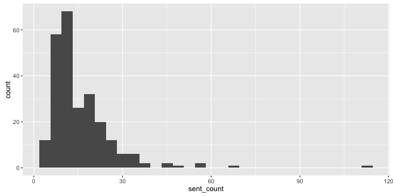
# 文書毎の文数
knbc_raw %>%
dplyr::group_by(did) %>%
dplyr::summarize(sent_count = max(sid)) %>%
ggplot2::ggplot(data =., ggplot2::aes(x = sent_count)) + ggplot2::geom_histogram()
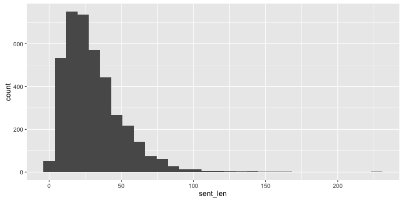
# ひとつの文の長さ
knbc_raw %>%
dplyr::mutate(sent_len = stringr::str_length(string = .$text)) %>%
ggplot2::ggplot(data =., ggplot2::aes(x = sent_len)) + ggplot2::geom_histogram()
# 各文から名詞と形容詞を抽出して、ファイルに書き出し
knbc_raw %>%
  dplyr::select(-gids) %>%
  dplyr::rowwise(data = .) %>%
  dplyr::mutate(text = extractContent(text = text, extract_pattern = "名詞|形容詞")) %>%
  readr::write_csv(path = SET_STAGING_FILE)
寄り道
コーパスファイルの読み込みに{chunked}を試したかったが(大規模テキストデータを一部分ずつ読み込んで処理するパッケージ)、EUC-JPが対応できなかったため、上記で各文から名詞と形容詞を抽出したファイルを読み込む実験。
# 単語頻度を集計に{chunked}を試す
knbc_chunked_corpus <- chunked::read_table_chunkwise(
  file = SET_STAGING_FILE, sep = ",", chunk_size = 500,
  header = TRUE
)

# while文を回す方法しか思い当たらなかったので、いい感じに対処する方法を要調査
knbc <- list()
knbc_chunk <- "NULL"
while (!is.null(x = knbc_chunk)) {
  knbc_chunk <- knbc_chunked_corpus$next_chunk(cmds = NULL)
  if (!is.null(x = knbc_chunk)) {
    knbc <- dplyr::bind_rows(
      knbc, knbc_chunk %>%
        tidytext::unnest_tokens_(output_col = "word", input_col = "text") %>%
        dplyr::count(word, sort = TRUE)
    )
  }
}

> knbc %>%
  dplyr::group_by(word) %>%
  dplyr::summarize(n = sum(n)) %>%
  dplyr::arrange(dplyr::desc(x = n))
# A tibble: 5,124 × 2
    word     n
   <chr> <int>
1     の   713
2   こと   475
3     人   321
4   携帯   317
5   京都   289
6     私   237
7   電話   224
8   よう   216
9   もの   198
10  観光   158
テキストを読み込み書き出すまでを一連の流れでやるときにはいいかもれないが、iterators::ireadLinesと使い分けがよくわからない。
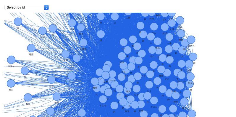
共起ネットワーク
{tidytext}と{widyr}で提供されている関数を組み合わせて共起頻度を集計し、{visNetwork}で共起ネットワークを作成。
knbc_corpus <- readr::read_csv(
  file = SET_STAGING_FILE,
  col_types = list(
    did = readr::col_integer(), sid = readr::col_integer(), text = readr::col_character()
  )
) %>%
  tidyr::drop_na()

> knbc_corpus %>%
  dplyr::filter(did == 1 & sid == 1)
# A tibble: 1 × 3
    did   sid                                                 text
  <int> <int>                                                <chr>
1     1     1 今さら\t接頭\t句\tない\t今さら\t私\tプリペイド\t携帯

# tri-gram
> knbc_corpus %>%
  tidytext::unnest_tokens_(output_col = "ngram", input_col = "text", token = "ngrams", n = 3) %>%
  dplyr::filter(did == 1 & sid == 1)
# A tibble: 6 × 3
    did   sid                ngram
  <int> <int>                <chr>
1     1     1       今さら 接頭 句
2     1     1         接頭 句 ない
3     1     1       句 ない 今さら
4     1     1       ない 今さら 私
5     1     1 今さら 私 プリペイド
6     1     1   私 プリペイド 携帯

# skip-gram
> knbc_corpus %>%
  tidytext::unnest_tokens_(output_col = "ngram", input_col = "text", token = "skip_ngrams", n = 3, k = 2) %>%
  dplyr::filter(did == 1 & sid == 1)
# A tibble: 12 × 3
     did   sid                  ngram
   <int> <int>                  <chr>
1      1     1 今さら ない プリペイド
2      1     1       接頭 今さら 携帯
3      1     1       今さら 句 今さら
4      1     1           接頭 ない 私
5      1     1   句 今さら プリペイド
6      1     1           ない 私 携帯
7      1     1         今さら 接頭 句
8      1     1           接頭 句 ない
9      1     1         句 ない 今さら
10     1     1         ない 今さら 私
11     1     1   今さら 私 プリペイド
12     1     1     私 プリペイド 携帯


# 文レベルでの共起頻度
knbc_co <- knbc_corpus %>%
  tidytext::unnest_tokens_(output_col = "word", input_col = "text", token = "words") %>%
  dplyr::anti_join(y = dplyr::data_frame(word = SET_STOP_WORD), by = "word") %>%
  widyr::pairwise_count(item = word, feature = sid, diag = FALSE, upper = FALSE) %>%
  dplyr::arrange(dplyr::desc(n))

# 共起頻度の頻度
> co_freq <- table(knbc_co$n) %>%
  print

      1       2       3       4       5       6       7       8       9      10      11      12
2547815  425269  150040   69181   37289   22272   14126    9336    6042    4215    2986    2165
     13      14      15      16      17      18      19      20      21      22      23      24
   1448    1050     780     561     357     266     206     141     112      66      60      36
     25      26      27      28      29      30      33
     29      18      14       4       5       2       1


# 共起ネットワークを可視化(頻度の累積相対度数(下位30%)を切り捨て)
knbc_co_net <- visNetwork::toVisNetworkData(
  igraph = igraph::graph.data.frame(
    d = knbc_co %>%
      dplyr::filter(n > which.max(x = dplyr::cume_dist(x = co_freq) < 0.70)) %>%
      dplyr::rename(from = item1, to = item2, value = n)
  ),
  idToLabel = TRUE
)
visNetwork::visNetwork(
  nodes = knbc_co_net$nodes, edges = knbc_co_net$edges,
  width = 900, height = 1200
) %>%
  visNetwork::visOptions(
    highlightNearest = TRUE, nodesIdSelection = TRUE
  ) %>%
  visNetwork::visIgraphLayout(layout = "layout_nicely") %>%
  visNetwork::visPhysics(stabilization = TRUE)
文書間の距離
{tidytext}と{widyr}で提供されている関数を組み合わせて、TF-IDFを素性にテキスト間の距離を算出。ここではドキュメントレベルで距離を出しているが、文レベルで距離の算出も引数を変えることで可能。
# 文書毎の単語頻度(ストップワード除去)
knbc_doc_word_cnt <- knbc_corpus %>%
  tidytext::unnest_tokens_(output_col = "word", input_col = "text", token = "words") %>%
  dplyr::anti_join(y = dplyr::data_frame(word = SET_STOP_WORD), by = "word") %>%
  dplyr::group_by(did, word) %>%
  dplyr::summarize(freq = n()) %>%
  dplyr::ungroup()

# 上位10単語を表示
> knbc_doc_word_cnt %>%
  dplyr::arrange(dplyr::desc(x = freq)) %>%
  dplyr::top_n(n = 10, wt = freq)
# A tibble: 10 × 3
     did   word  freq
   <int>  <chr> <int>
1     56   神社    25
2     69   電話    20
3    200 うどん    20
4     69   携帯    19
5    110   離宮    18
6      1   携帯    16
7     70     局    16
8     70   交通    16
9     70     市    16
10   197   餃子    16

# TF-IDF
> knbc_doc_tfidf <- knbc_doc_word_cnt %>%
  tidytext::bind_tf_idf_(term_col = "word", document_col = "did", n_col = "freq")

# IDF上位10単語を表示
> knbc_doc_tfidf %>%
  dplyr::arrange(dplyr::desc(x = tf_idf)) %>%
  dplyr::top_n(n = 10, wt = idf)
# A tibble: 2,962 × 6
     did       word  freq         tf      idf    tf_idf
   <int>      <chr> <int>      <dbl>    <dbl>     <dbl>
1    231 さつまいも     3 0.10000000 5.517453 0.5517453
2    141   なぎなた     3 0.08823529 5.517453 0.4868341
3    100     真如堂     4 0.08333333 5.517453 0.4597877
4     97       ケイ     5 0.07692308 5.517453 0.4244195
5    154     レタス    11 0.07534247 5.517453 0.4156985
6    172         傷     3 0.07317073 5.517453 0.4037161
7    215         九     5 0.06944444 5.517453 0.3831565
8     70         局    16 0.06400000 5.517453 0.3531170
9    238       動物     4 0.06349206 5.517453 0.3503145
10   220       味噌     7 0.06194690 5.517453 0.3417891
# ... with 2,952 more rows

# TF-IDF上位10単語を表示
> knbc_doc_tfidf %>%
  dplyr::arrange(dplyr::desc(x = tf_idf)) %>%
  dplyr::top_n(n = 20, wt = tf_idf)
# A tibble: 20 × 6
     did         word  freq         tf      idf    tf_idf
   <int>        <chr> <int>      <dbl>    <dbl>     <dbl>
1    189         焼肉     5 0.15625000 4.824306 0.7537978
2    110         離宮    18 0.14285714 4.824306 0.6891865
3    238           ぃ    11 0.17460317 3.725693 0.6505179
4    103         広告     7 0.14000000 4.418841 0.6186377
5    232       カフェ    12 0.16666667 3.571543 0.5952571
6    200       うどん    20 0.12820513 4.418841 0.5665180
7    231   さつまいも     3 0.10000000 5.517453 0.5517453
8    219 チャーシュー     4 0.10810811 4.824306 0.5215466
9    132         入力    12 0.13333333 3.908015 0.5210687
10   218         弁当     6 0.10714286 4.824306 0.5168899
11   178         充電     5 0.12500000 4.131159 0.5163948
12    44       ボタン     4 0.11428571 4.418841 0.5050104
13   141     なぎなた     3 0.08823529 5.517453 0.4868341
14   220       おでん    11 0.09734513 4.824306 0.4696227
15   169       パフェ     5 0.12500000 3.725693 0.4657117
16   100       真如堂     4 0.08333333 5.517453 0.4597877
17   197         餃子    16 0.09467456 4.824306 0.4567390
18   112         返信     7 0.12727273 3.571543 0.4545600
19   237           ぃ     6 0.12000000 3.725693 0.4470832
20    97         ケイ     5 0.07692308 5.517453 0.4244195


# 文書間の距離(文書毎にTF-IDFが上位の10語に限定)
knbc_doc_dist <- knbc_doc_tfidf %>%
  dplyr::group_by(did) %>%
  dplyr::top_n(n = 10, wt = tf_idf) %>%
  dplyr::ungroup() %>%
  widyr::pairwise_dist(item = did, feature = word, value = tf_idf, method = "euclidean", upper = FALSE) %>%
  dplyr::arrange(distance)

# 一番近い文書同士で共通して出現する単語を表示
dplyr::inner_join(
  x = knbc_doc_tfidf %>%
    dplyr::filter(did == knbc_doc_dist$item1[1]) %>%
    dplyr::select(word, did, tf_idf) %>%
    dplyr::arrange(dplyr::desc(x = tf_idf)),
  y = knbc_doc_dist %>%
    dplyr::filter(item1 == knbc_doc_dist$item1[1]) %>%
    dplyr::top_n(n = 1, wt = -distance) %>%
    dplyr::select(did = item2) %>%
    dplyr::left_join(y = knbc_doc_tfidf) %>%
    dplyr::select(word, did, tf_idf) %>%
    dplyr::arrange(dplyr::desc(x = tf_idf)),
  by = c("word")
) %>%
  as.data.frame()
Joining, by = "did"
     word did.x    tf_idf.x did.y    tf_idf.y
1    卒業    52 0.021661008   115 0.018174114
2    あと    52 0.021160556   115 0.011836149
3    是非    52 0.020764783   115 0.017422160
4    多い    52 0.016394187   115 0.009170082
5      ん    52 0.013348896   115 0.005600025
6      昔    52 0.008367429   115 0.014040954
7      前    52 0.007990222   115 0.006703991
8    今日    52 0.006800579   115 0.011411703
9      笑    52 0.006352466   115 0.010659748
10   どこ    52 0.005874841   115 0.019716540
11     目    52 0.005874841   115 0.009858270
12     年    52 0.004666947   115 0.015662731
13   時間    52 0.004443223   115 0.037279728
14 ところ    52 0.004389883   115 0.007366438
15     人    52 0.003914336   115 0.022989564
16     一    52 0.003488270   115 0.011706973
17   いい    52 0.002894373   115 0.004856899
18   ない    52 0.002862946   115 0.004804163
抽出されたワードが望ましいものが少なそうなので、ストップワードをもっと定義したり、形態素解析に用いる辞書をNeologdに変えた方が適した結果になりそう。また、widyr::pairwise_distの距離尺度はstat::distしか使えないので、proxy::distが使えるようになると嬉しい。
Latent Dirichlet Allocation(LDA)
文書毎の単語頻度のオブジェクトを{tm}のDTM(Document-Term-Matrix)やTDM(Term-Document-Matrix)に変換して、topicmodels::LDAを実行して結果を{LDAvis}で可視化。
# CAST Document-Term-Matrix
> knbc_dtm <- knbc_doc_word_cnt %>%
  tidytext::cast_dtm_(term_col = "word", document_col = "did", value_col = "freq") %>%
  print
<<DocumentTermMatrix (documents: 249, terms: 5118)>>
Non-/sparse entries: 15776/1258606
Sparsity           : 99%
Maximal term length: 13
Weighting          : term frequency (tf)

> tidytext::tidy(x = knbc_dtm)
# A tibble: 15,776 × 3
   document     term count
      <chr>    <chr> <dbl>
1         1   com     1
2         2   com     1
3        46   com     1
4        69   com     1
5         1 http     1
6         2 http     2
7        35 http     1
8        46 http     1
9        69 http     3
10       92 http     1
# ... with 15,766 more rows


# CAST Term-Document-Matrix
> knbc_tdm <- knbc_doc_word_cnt %>%
  tidytext::cast_tdm_(term_col = "word", document_col = "did", value_col = "freq") %>%
  print
<<TermDocumentMatrix (terms: 5118, documents: 249)>>
Non-/sparse entries: 15776/1258606
Sparsity           : 99%
Maximal term length: 13
Weighting          : term frequency (tf)

> tidytext::tidy(x = knbc_tdm)
# A tibble: 15,776 × 3
                   term document count
                  <chr>    <chr> <dbl>
1                com        1     1
2              http        1     1
3              mixi        1     1
4  prepaidfan        1     1
5                  sa        1     1
6      softbank        1     1
7      vodafone        1     1
8                web        1     1
9                www        1     1
10               いくつ        1     1
# ... with 15,766 more rows
# KNBCコーパスはGourmet, Keitai, Kyoto, Sportsについて書かれたコーパスなので、トピック数を4に指定して実行
knbc_dtm_lda <- topicmodels::LDA(x = knbc_dtm, k = 4, method = "Gibbs")

# 単語の生成確率が一番高いトピック
topic_term <- tidytext::tidy(knbc_dtm_lda, matrix = "beta") %>%
  dplyr::group_by(term) %>%
  dplyr::top_n(n = 1, wt = beta) %>%
  dplyr::arrange(topic) %>%
  ungroup()

# 各トピック毎に生成確率が高い上位10単語を表示
> topic_term %>%
  dplyr::group_by(topic) %>%
  dplyr::top_n(n = 10, wt = beta) %>%
  as.data.frame()
   topic     term        beta
1      1       一 0.014223022
2      1       人 0.035533876
3      1       年 0.006961546
4      1       さ 0.010592284
5      1     観光 0.024799520
6      1     京都 0.045636800
7      1     時間 0.011539433
8      1       寺 0.009645135
9      1     神社 0.009171560
10     1     清水 0.007592978
11     2     機能 0.009552115
12     2     携帯 0.050398932
13     2       今 0.010823612
14     2     自分 0.009869990
15     2       的 0.009711052
16     2     電話 0.035617788
17     2     いい 0.010982549
18     2       気 0.008916367
19     2     とき 0.011777234
20     2   メール 0.022743889
21     3     それ 0.011788188
22     3     ない 0.017929646
23     3       何 0.010252823
24     3       前 0.011105804
25     3       中 0.010082227
26     3       っ 0.015029513
27     3       ん 0.025435873
28     3     好き 0.013494149
29     3     しく 0.009741035
30     3     大学 0.010082227
31     4       円 0.013884887
32     4       方 0.006861403
33     4       く 0.010283100
34     4       京 0.009202564
35     4       日 0.011543726
36     4     さん 0.007581761
37     4 おいしい 0.007941939
38     4       店 0.014425155
39     4     料理 0.011363636
40     4       味 0.007581761

# 各トピック毎に生成確率が高い単語を可視化
ggplot2::ggplot(
  tidytext::tidy(knbc_dtm_lda) %>%
    dplyr::filter(beta > 0.010) %>%
    dplyr::mutate(term = reorder(term, beta)),
  ggplot2::aes(term, beta)
) + ggplot2::geom_bar(stat = "identity") + ggplot2::facet_wrap(~ topic, scales = "free") +
  ggplot2::theme(axis.text.x = ggplot2::element_text(angle = 90, size = 15)) +
  # Macでの日本語文字列表示用
  ggplot2::theme_bw(base_family = "HiraKakuProN-W3")
# 各テキストでひとつのトピックを選ぶ
> dplyr::left_join(
  x = tidytext::tidy(knbc_dtm_lda, matrix = "gamma") %>%
    dplyr::group_by(document) %>%
    dplyr::arrange(gamma) %>%
    dplyr::top_n(n = 1, wt = gamma) %>%
    ungroup() %>%
    dplyr::mutate(document = as.integer(x = document)) %>%
    dplyr::select(-gamma),
  y = knbc_domain,
  by = c("document" = "did")
) %>%
  dplyr::select(topic, domain) %>%
  table %>%
  print
     domain
topic Gourmet Keitai Kyoto Sports
    1       3      1    72      1
    2       0     70     1      1
    3       8      7     9     20
    4      48      1    13      0


# tidytext::augmentでも同じ結果になると思ったが、微妙に異なる(要確認)
dplyr::left_join(
  x = tidytext::augment(x = knbc_dtm_lda) %>%
    dplyr::mutate(document = as.integer(x = .$document)) %>%
    dplyr::group_by(document, .topic) %>%
    dplyr::summarize(cnt = n()) %>%
    dplyr::arrange(document, cnt) %>%
    dplyr::top_n(n = 1, wt = cnt) %>%
    dplyr::select(document, .topic),
  y = knbc_domain,
  by = c("document" = "did")
) %>%
  dplyr::ungroup() %>%
  dplyr::select(.topic, domain) %>%
  table
      domain
.topic Gourmet Keitai Kyoto Sports
     1       4      1    66      1
     2       0     70     3      2
     3       8      7    12     20
     4      45      1    14      0


# {LDAvis}で可視化
lda_posterior <- topicmodels::posterior(object = knbc_dtm_lda)
most_probable_topic_word <- knbc_dtm_lda @ wordassignments
lda_json <- LDAvis::createJSON(
  phi = lda_posterior$terms,
  theta = lda_posterior$topics,
  vocab = colnames(x = lda_posterior$terms),
  doc.length = slam::row_sums(x = most_probable_topic_word, na.rm = TRUE),
  term.frequency = slam::col_sums(x = most_probable_topic_word, na.rm = TRUE)
)
LDAvis::serVis(json = lda_json, out.dir = "knbc_lda", open.browser = TRUE)
(トピック毎のスクリーンショット)


可視化結果とモデルによるトピックの対応が取れていないように見えるので(モデルによる結果は「京都、携帯、スポーツ、グルメ」の順のようだが、可視化結果は「グルメ、スポーツ、携帯、京都」に見える)、要確認。
GloVe
{Matrix}クラスのオブジェクトに変換してから{text2vec}を実行(直接だとエラーが出る)。作成されたベクトルを用いてアナロジー(類推)を試す。
# no method or default for coercing “DocumentTermMatrix” to “dgCMatrix”
# knbc_tcm <- textmineR::Dtm2Tcm(dtm = as(object = knbc_dtm, Class = "dgCMatrix"))
knbc_tcm <- textmineR::Dtm2Tcm(dtm = as(object = knbc_dtm, Class = "Matrix"))
knbc_glove_fit <- text2vec::glove(
  tcm = knbc_tcm, word_vectors_size = 50,
  num_iters = 50, x_max = 10, convergence_threshold = 0.005,
  verbose = FALSE
)
word_vectors <- knbc_glove_fit$word_vectors[[1]] + knbc_glove_fit$word_vectors[[2]]
rownames(x = word_vectors) <- rownames(x = knbc_tcm)
word_vectors_norm <- sqrt(x = rowSums(x = word_vectors ^ 2))

# アナロジー
query <- word_vectors["ラーメン", , drop = FALSE] + word_vectors["餃子", , drop = FALSE]

cos_dist <- text2vec:::cosine(
  m_query = query, m_source = word_vectors, m_source_norm = word_vectors_norm
)
> head(sort(x = cos_dist[1, ], decreasing = TRUE), n = 10)
      餃子   ラーメン       直伝         具         母       九州         棒 インパクト     我が家
 0.7830368  0.6812339  0.6218219  0.5890876  0.5718114  0.5650479  0.5609208  0.5578002  0.5537876
  しょうゆ
 0.5481026
使用したコーパス量も多くないので、あまりいい結果にはなっていない。Wikipediaコーパスなどで真面目に試したい。
まとめ
KNBCコーパスを対象に、モダンなRの書き方でテキスト解析を行いました。既存のパッケージを組み合わせることで、テキスト処理からTF-IDFや共起頻度(ネットワーク作成)、LDAやGloVeまでを手軽に実行できましたが、ストップワードの追加や形態素解析辞書の変更、コーパス増強など、もう少し言語処理的な工夫が必要です。このあたりはまだまだ課題と言えます。
しかしながら、Rでのテキスト処理もしやすい環境になってきていると思いますので、興味をもった方はぜひ挑戦していただきたいです。
GloVeの実行で今回用いた{text2vec}は以前にword2vecの実行で使用した{wordVectors}よりも実装が良さげで(日本語テキストにも対応している)、大規模なテキスト処理にも活用できそうなので個人的にはこちらを使っていきたいです。
参考
- Rで始める文字列処理
- {stringr}/{stringi}とbaseの文字列処理について
- Introduction to tidytext
- Widen, process, and re-tidy a dataset
- トピックモデルことはじめ
- A topic model for movie reviews
- [翻訳] text2vec vignette: text2vecパッケージによるテキスト分析
実行環境
> devtools::session_info()
Session info ----------------------------------------------------------------------------------------
 setting  value
 version  R version 3.3.1 (2016-06-21)
 system   x86_64, darwin13.4.0
 ui       RStudio (0.99.903)
 language (EN)
 collate  ja_JP.UTF-8
 tz       Asia/Tokyo
 date     2016-09-12

Packages --------------------------------------------------------------------------------------------
 package      * version    date       source
 assertthat     0.1        2013-12-06 CRAN (R 3.3.1)
 broom          0.4.1      2016-06-24 CRAN (R 3.3.0)
 chron          2.3-47     2015-06-24 CRAN (R 3.3.1)
 chunked      * 0.3        2016-06-24 CRAN (R 3.3.0)
 codetools      0.2-14     2015-07-15 CRAN (R 3.3.1)
 colorspace     1.2-6      2015-03-11 CRAN (R 3.3.1)
 data.table     1.9.6      2015-09-19 CRAN (R 3.3.1)
 DBI            0.5        2016-08-11 cran (@0.5)
 devtools       1.12.0     2016-06-24 CRAN (R 3.3.0)
 digest         0.6.9      2016-01-08 CRAN (R 3.3.0)
 dplyr        * 0.5.0      2016-06-24 CRAN (R 3.3.1)
 foreach        1.4.3      2015-10-13 CRAN (R 3.3.1)
 ggplot2      * 2.1.0      2016-03-01 CRAN (R 3.3.1)
 gtable         0.2.0      2016-02-26 CRAN (R 3.3.1)
 htmltools      0.3.5      2016-03-21 CRAN (R 3.3.1)
 htmlwidgets    0.6        2016-02-25 CRAN (R 3.3.1)
 iterators      1.0.8      2015-10-13 CRAN (R 3.3.1)
 janeaustenr    0.1.1      2016-06-20 CRAN (R 3.3.0)
 jsonlite       1.0        2016-07-01 CRAN (R 3.3.0)
 lattice        0.20-33    2015-07-14 CRAN (R 3.3.1)
 LDAvis       * 0.3.2      2015-10-24 CRAN (R 3.3.0)
 magrittr       1.5        2014-11-22 CRAN (R 3.3.1)
 Matrix       * 1.2-6      2016-05-02 CRAN (R 3.3.1)
 memoise        1.0.0      2016-01-29 CRAN (R 3.3.0)
 mnormt         1.5-4      2016-03-09 CRAN (R 3.3.0)
 modeltools     0.2-21     2013-09-02 CRAN (R 3.3.1)
 munsell        0.4.3      2016-02-13 CRAN (R 3.3.1)
 nlme           3.1-128    2016-05-10 CRAN (R 3.3.1)
 NLP            0.1-9      2016-02-18 CRAN (R 3.3.1)
 pacman       * 0.4.1      2016-03-30 CRAN (R 3.3.0)
 plyr           1.8.4      2016-06-08 CRAN (R 3.3.1)
 psych          1.6.6      2016-06-28 CRAN (R 3.3.0)
 purrr        * 0.2.2      2016-06-18 CRAN (R 3.3.1)
 R6             2.1.3      2016-08-19 cran (@2.1.3)
 Rcpp         * 0.12.7     2016-09-05 cran (@0.12.7)
 RcppParallel   4.3.19     2016-05-05 CRAN (R 3.3.1)
 RcppProgress   0.2.1      2015-01-09 CRAN (R 3.3.0)
 readr        * 1.0.0      2016-08-03 cran (@1.0.0)
 reshape2       1.4.1      2014-12-06 CRAN (R 3.3.1)
 rsconnect      0.4.3      2016-08-13 Github (rstudio/rsconnect@1665cb8)
 scales         0.4.0      2016-02-26 CRAN (R 3.3.1)
 slam           0.1-37     2016-08-05 cran (@0.1-37)
 SnowballC      0.5.1      2014-08-09 CRAN (R 3.3.1)
 stringi        1.1.1      2016-05-27 CRAN (R 3.3.1)
 stringr        1.1.0      2016-08-19 cran (@1.1.0)
 text2vec     * 0.3.0      2016-03-31 CRAN (R 3.3.0)
 textmineR    * 2.0.2      2016-06-06 CRAN (R 3.3.0)
 tibble       * 1.2        2016-08-26 cran (@1.2)
 tidyr        * 0.6.0      2016-08-12 cran (@0.6.0)
 tidytext     * 0.1.1      2016-06-25 CRAN (R 3.3.0)
 tidyverse    * 0.0.0.9000 2016-09-07 Github (hadley/tidyverse@7149f49)
 tm             0.6-2      2015-07-03 CRAN (R 3.3.0)
 tokenizers     0.1.2      2016-04-14 CRAN (R 3.3.0)
 topicmodels  * 0.2-4      2016-05-23 CRAN (R 3.3.0)
 visNetwork   * 1.0.1      2016-06-20 CRAN (R 3.3.0)
 widyr        * 0.0.0.9000 2016-09-07 Github (dgrtwo/widyr@46c508a)
 withr          1.0.2      2016-06-20 CRAN (R 3.3.0)