R言語 - 回帰モデルを使った分析

はじめに

　この Tips では、回帰分析を紹介しています。サンプルの分析では、ランニングのトレーニング目標を考えるために、過去のトレーニング量に対して、回帰分析としていくつかのモデル式を適用し、モデルの良さを評価した上で、今後のランニング目標を決定しています。モデルは、累乗、指数、漸近指数、ロジスティック曲線、ゴンペルツ曲線を当てはめて、モデルの評価には、AIC(赤池情報量規準)を使用しました。

モデル名	モデル式
累乗モデル	$y=ax^b$
指数モデル	$y=ab^x$
漸近指数モデル	$y=Asymp+(R0-Asymp)exp(-exp(lrc)*x)$
ロジスティック曲線モデル	$y=Asym/(1+exp((xmid-x)/scal))$
ゴンペルツ曲線モデル	$y=Asym*exp(-b2*b3^x)$

データの作成

サンプルデータ

# 過去のトレーニング期間のデータを作成
timeFrame <- c( "Sep-12", "Oct-12", "Nov-12", "Dec-12", "Jan-13", "Feb-13", "Mar-13", "Apr-13", "May-13", "Jun-13", "Jul-13", "Aug-13", "Sep-13", "Oct-13", "Nov-13", "Dec-13", "Jan-14", "Feb-14", "Mar-14", "Apr-14", "May-14", "Jun-14", "Jul-14", "Aug-14", "Sep-14", "Oct-14", "Nov-14", "Dec-14", "Jan-15", "Feb-15", "Mar-15", "Apr-15", "May-15", "Jun-15", "Jul-15", "Aug-15", "Sep-15", "Oct-15", "Nov-15", "Dec-15" )
# 過去のトレーニング期間の回数データを作成
trainingSequence <- as.numeric(c(1:length(timeFrame)))
# 過去のトレーニング量(走行距離(Km))のデータを作成
runDistance <- as.numeric(c( "65", "33", "31.4", "55.6", "47", "77", "100.3", "50.35", "77.6", "80", "81.5", "53", "126.5", "85.1", "96", "128.8", "75.7", "80.6", "91.1", "83.1", "51", "63.5", "64.2", "63.1", "74.8", "86", "136", "116", "125", "105", "105", "93", "95.5", "85", "88", "100", "105.5", "89", "92", "117" ))
# トレーニングログをデータフレームとして作成
trainingLog <- data.frame( trainingSequence, timeFrame, runDistance ) 

累乗モデルへの当てはめ

R

# nlsファンクションを使って、累乗モデルに当てはめる
powerModel <- nls( trainingLog$runDistance~a*trainingLog$trainingSequence^b, start=list( a=1, b=1 ))
# 分析結果の確認
summary ( powerModel ) 

分析結果例

Formula: trainingLog$runDistance ~ a * trainingLog$trainingSequence^b
Parameters: # パラメータ推定値、標準誤差、t 値、p 値
  Estimate Std. Error t value Pr(>|t|)    
a 44.22670    7.97657   5.545  2.4e-06 ***
b  0.22765    0.05831   3.904 0.000375 ***
---
Signif. codes:  0 ‘***’ 0.001 ‘**’ 0.01 ‘*’ 0.05 ‘.’ 0.1 ‘ ’ 1
Residual standard error: 20.92 on 38 degrees of freedom
Number of iterations to convergence: 8 
Achieved convergence tolerance: 6.662e-06

　累乗モデルからパラメータaとbの推定値を得られたので、次の式を推定することができました。

累乗モデル

トレーニング量=44.22670*トレーニング回数^{0.22765}

指数モデルへの当てはめ

R

# nlsファンクションを使って、指数モデルに当てはめる
exponentModel <- nls( trainingLog$runDistance~a*b^trainingLog$trainingSequence, start=list( a=1, b=1 ))
# 分析結果の確認
summary ( exponentModel ) 

分析結果例

Formula: trainingLog$runDistance ~ a * b^trainingLog$trainingSequence
Parameters: # パラメータ推定値、標準誤差、t 値、p 値
   Estimate Std. Error t value Pr(>|t|)    
a 63.278770   6.040147   10.48 9.22e-13 ***
b  1.013546   0.003649  277.72  < 2e-16 ***
---
Signif. codes:  0 ‘***’ 0.001 ‘**’ 0.01 ‘*’ 0.05 ‘.’ 0.1 ‘ ’ 1
Residual standard error: 21.82 on 38 degrees of freedom
Number of iterations to convergence: 8 
Achieved convergence tolerance: 2.917e-06

　指数モデルからパラメータaとbの推定値を得られたので、次の式を推定することができました。

指数モデル

トレーニング量=63.27877*1.013546^{トレーニング回数}

漸近指数モデルへの当てはめ

R

# nlsファンクションを使って、漸近指数モデルに当てはめる
asymptoteModel <- nls( trainingLog$runDistance~SSasymp( trainingLog$trainingSequence, Asymp, R0, lrc ))
# 分析結果の確認
summary ( asymptoteModel ) 

分析結果例

Formula: trainingLog$runDistance ~ SSasymp(trainingLog$trainingSequence, Asymp, R0, lrc)
Parameters: # パラメータ推定値、標準誤差、t 値、p 値
      Estimate Std. Error t value Pr(>|t|)    
Asymp  99.1614     8.8335  11.226 1.79e-13 ***
R0     38.1248    16.4724   2.314  0.02630 *  
lrc    -2.3442     0.6049  -3.875  0.00042 ***
---
Signif. codes:  0 ‘***’ 0.001 ‘**’ 0.01 ‘*’ 0.05 ‘.’ 0.1 ‘ ’ 1
Residual standard error: 21.11 on 37 degrees of freedom
Number of iterations to convergence: 0 
Achieved convergence tolerance: 2.524e-06

　漸近指数モデルからパラメータ Asymp、R0、lrc を得られたので、次の式を推定することができました。

漸近指数モデル

トレーニング量=99.1614+(38.1248-99.1614)exp(-exp(-2.3442)トレーニング回数

ロジスティック曲線モデルへの当てはめ

R

# nlsファンクションを使って、ロジスティック曲線モデルを当てはめる
logisticsModel <- nls( trainingLog$runDistance ~ SSlogis(trainingLog$trainingSequence, Asym, xmid, scal ))
# 分析結果の確認
summary( logisticsModel )

分析結果例

Formula: trainingLog$runDistance ~ SSlogis(trainingLog$trainingSequence, Asym, xmid, scal)
Parameters: # パラメータ推定値、標準誤差、t 値、p 値
     Estimate Std. Error t value Pr(>|t|)    
Asym   95.608      5.708  16.749   <2e-16 ***
xmid    1.854      2.396   0.774   0.4438    
scal    5.774      2.923   1.976   0.0557 .  
---
Signif. codes:  0 ‘***’ 0.001 ‘**’ 0.01 ‘*’ 0.05 ‘.’ 0.1 ‘ ’ 1
Residual standard error: 21.18 on 37 degrees of freedom
Number of iterations to convergence: 2 
Achieved convergence tolerance: 8.752e-06

　ロジスティック曲線モデルからパラメータ Asym、xmid、scal を得られたので、次の式を推定することができました。

ロジスティック曲線

トレーニング量=95.608/( 1+exp(( 1.854 - トレーニング回数 )/5.774))

ゴンペルツ曲線モデルへの当てはめ

R

# nlsファンクションを使って、ゴンペルツ曲線モデルを当てはめる
GompertzModel <- nls( trainingLog$runDistance~SSgompertz( trainingLog$trainingSequence, Asym, b2, b3 ))
# 分析結果の確認
summary ( GompertzModel ) 

分析結果例

Formula: trainingLog$runDistance ~ SSgompertz(trainingLog$trainingSequence, Asym, b2, b3)
Parameters: # パラメータ推定値、標準誤差、t 値、p 値
     Estimate Std. Error t value Pr(>|t|)    
Asym 97.15226    6.86999  14.142   <2e-16 ***
b2    0.89681    0.33065   2.712   0.0101 *  
b3    0.87785    0.06143  14.290   <2e-16 ***
---
Signif. codes:  0 ‘***’ 0.001 ‘**’ 0.01 ‘*’ 0.05 ‘.’ 0.1 ‘ ’ 1
Residual standard error: 21.14 on 37 degrees of freedom
Number of iterations to convergence: 3 
Achieved convergence tolerance: 4.49e-06

　ゴンペルツ曲線モデルからパラメータ Asym、b2、b3 を得られたので、次の式を推定することができました。

ゴンペルツ曲線モデル

トレーニング量=97.15226*exp(-0.89681*0.87785^{トレーニング回数})

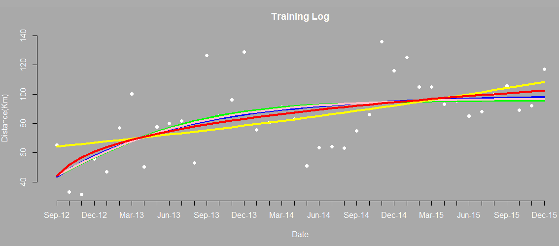
グラフを確認する

　式を推定できたので、トレーニングログの散布図上に、それぞれの式をグラフ描画します。

R

# トレーニングログを描画
par( bg="darkgray" , col="white", col.axis="white", col.lab="white", col.main="white", col.sub="white")
plot (trainingLog$trainingSequence, trainingLog$runDistance, pch=19, axes = FALSE, main="Training Log", ylab="Distance(Km)", xlab="Date")
axis(side=1, at = trainingLog$trainingSequence, labels = trainingLog$timeFrame)
axis(side=2)
par( new=TRUE ) 
# 累乗モデルへの当てはめを描画
lines(trainingLog$trainingSequence, 44.22670*trainingLog$trainingSequence^(0.22765), col = "red", lwd=4 ) 
# 指数モデルへの当てはめを描画
lines(trainingLog$trainingSequence, 63.278770 * 1.013546^trainingLog$trainingSequence, col = "yellow", lwd=4 ) 
# 漸近指数モデルへの当てはめを描画
lines(trainingLog$trainingSequence,( 99.1614+(38.1248-99.1614)*exp(-exp(-2.3442)*trainingLog$trainingSequence) ) , col = "blue", lwd=4 ) 
# ロジスティック曲線モデルへの当てはめを描画
lines(trainingLog$trainingSequence,( 95.608/(1 + exp(( 1.854 - trainingLog$trainingSequence )/5.774)) ) , col = "green", lwd=4 )
# ゴンペルツ曲線モデルへの当てはめを描画
lines(trainingLog$trainingSequence,( 97.15226*exp(-0.89681*0.87785^trainingLog$trainingSequence )) , col = "pink", lwd=4)

AICでモデルを評価する

　最後に、AIC(赤池情報量規準)で統計モデルの良さを評価します。具体的には AIC ファンクションを実行して、相対的に値が最小のモデルを選択します。

R

# 累乗モデル(赤色のグラフ)
AIC(powerModel)
# 指数モデル(黄色のグラフ)
AIC(exponentModel)
# 漸近指数モデル(青色のグラフ)
AIC(asymptoteModel)
# ロジスティック成長モデル(緑色のグラフ)
AIC(logisticsModel)
# ゴンペルツ成長モデル(桃色のグラフ)
AIC(GompertzModel)

実行結果例

> # 累乗モデル(赤色のグラフ)
> AIC(powerModel)
[1] 360.7268
> # 指数モデル(黄色のグラフ)
> AIC(exponentModel)
[1] 364.08
> # 漸近指数モデル(青色のグラフ)
> AIC(asymptoteModel)
[1] 362.393
> # ロジスティック曲線モデル(緑色のグラフ)
> AIC(logisticsModel)
[1] 362.6532
> # ゴンペルツ曲線モデル(桃色のグラフ)
> AIC(GompertzModel)
[1] 362.5037

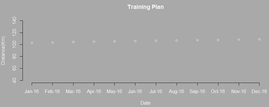
さいごに

　サンプルの分析では、グラフの確認とAICの評価から、累乗モデル(赤色のグラフ)による回帰モデルを選択して、今後のランニングのトレーニング目標を計画することにしました。具体的には次のような計画になりますが、年間の走行距離が約1272Kmという無理のない現実的なトレーニング目標になったと思います。

リファレンス

R 基本統計関数マニュアル
福岡大学 非線形回帰分析