Pythonで実装 PRML 第1章 ベイズ推定

前回に続いて、PRML1章から「1.2.6 ベイズ推定」の実装です。
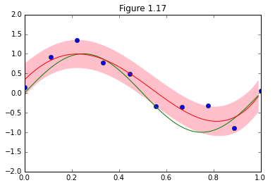
図1.17の再現ですが、M=9とした上で、予測分布の平均と±1σの範囲を示しています。

数式追ってるだけだと抽象的で、いまいちピンと来なかったんですが、
実装することで、(1.70)、(1.71)が分布を示すことが具体的に可視化されて腹に落ちました。
この予測精度が、前回の多項式曲線フィッティングとどう異なるのかは今回の例からは判断できませんが、
それぞれどのようなものかを理解する上では大変役立ちました。

実装の大まかな流れ

①求めたいのは予測分布(1.69)。

 p(t| x, {\bf x}, {\bf t}) = N(t| m(x), s^2(x)) (1.69)

②今回、基底関数は$\phi_i(x) = x^i$ for $i = 0,...M$ 。

③予測分布の平均、分散を求める式は下記の3つなので、これをそれぞれ実装して、予測範囲 $0.0<x<1.0$の分布を可視化する。

m(x) = \beta\phi(x)^{\bf T}{\bf S} \sum_{n=1}^N \phi(x_n)t_n(1.70)]

 s^2(x) = \beta^{-1} + \phi(x)^{\bf T} {\bf S} \phi(x)(1.71)

{\bf S}^{-1} = \alpha {\bf I} + \beta \sum_{n=1}^N \phi(x_n)\phi(x_n)^{\bf T}(1.72)

コード

import numpy as np
from numpy.linalg import inv
import pandas as pd
from pylab import *
import matplotlib.pyplot as plt

#From p31 the auther define phi as following
def phi(x):
    return np.array([x**i for i in xrange(M+1)]).reshape((M+1, 1))

#(1.70) Mean of predictive distribution
def m(x, x_train, y_train, S):
    sum = np.array(zeros((M+1, 1)))
    for n in xrange(len(x_train)):
        sum += np.dot(phi(x_train[n]), y_train[n])
    return Beta * phi(x).T.dot(S).dot(sum)


#(1.71) Variance of predictive distribution   
def s2(x, S):
    return 1.0/Beta + phi(x).T.dot(S).dot(phi(x))

#(1.72)
def S(x_train, y_train):
    I = np.identity(M+1)
    Sigma = np.zeros((M+1, M+1))
    for n in range(len(x_train)):
        Sigma += np.dot(phi(x_train[n]), phi(x_train[n]).T)
    S_inv = alpha*I + Beta*Sigma
    S = inv(S_inv)
    return S

if __name__ == "__main__":
    alpha = 0.005
    Beta = 11.1
    M = 9

    #Sine curve
    x_real = np.arange(0, 1, 0.01)
    y_real = np.sin(2*np.pi*x_real)

    ##Training Data
    N=10
    x_train = np.linspace(0, 1, 10)

    #Set "small level of random noise having a Gaussian distribution"
    loc = 0
    scale = 0.3
    y_train =  np.sin(2*np.pi*x_train) + np.random.normal(loc,scale,N)


    S = S(x_train, y_train)

    #Seek predictive distribution corespponding to entire x
    mean = [m(x, x_train, y_train, S)[0,0] for x in x_real]
    variance = [s2(x, S)[0,0] for x in x_real]
    SD = np.sqrt(variance)
    upper = mean + SD
    lower = mean - SD


    plot(x_train, y_train, 'bo')
    plot(x_real, y_real, 'g-')
    plot(x_real, mean, 'r-')
    fill_between(x_real, upper, lower, color='pink')
    xlim(0.0, 1.0)
    ylim(-2, 2)
    title("Figure 1.17")

結果