Pythonで実装 PRML 第1章 多項式曲線フィッティング

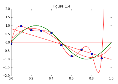
パターン認識と機械学習、第1章から「多項式多項式曲線フィッティング」の図の再現に取り組んでみます。
早速図1.4の再現から行ってみたいと思います。また、データの数を増やすことで、予測の正確性が増すことの確認を図1.6で行っています。

数学的にも実装上もまだまだそんなに難しくないので、淡々と実装してみました。
とりあえず、最初の第一歩。

実装の大まかな流れ

①(1.1)を実装。

 y(x, {\bf w}) = w_0 + w_1 x + w_1 x^2 + ...+ w_M x^M = \sum_{j=1}^M w_j x^M (1.1)

②(1.122)と(1.123)を満たす値を求めると二乗誤差関数(1.2)を最小化するパラメータ${\bf w}$の値が求まる。

E({\bf w}) = \frac{1}{2}  \sum_{n=1}^N \{{y({x_n, \bf x_n}) -t_n}^2 \}(1.2)

\sum_{j=0}^M {\bf A}_{ij} w_j = {\bf T}_i(1.122)

{\bf A}_i = \sum_{n=1}^N (x_n)^{i+j} (1.123)

{\bf T}_i = \sum_{n=1}^N (x_n)^i t_n (1.123)

コード

import numpy as np
import pandas as pd
from pylab import *
import matplotlib.pyplot as plt
#(1.1)
def y(x, W, M):
    Y = np.array([W[i] * (x ** i) for i in xrange(M+1)])
    return Y.sum()

#(1.2),(1.122),(1.123)
def E(x, t, M):
    A =np.zeros((M+1, M+1))
    for i in range(M+1):
        for j in range(M+1):
            A[i,j] = (x**(i+j)).sum()

    T = np.array([((x**i)*t).sum() for i in xrange(M+1)])
    return  np.linalg.solve(A, T)

if __name__ == "__main__":
    #Sine curve
    x_real = np.arange(0, 1, 0.01)
    y_real = np.sin(2*np.pi*x_real)

    ##Training Data
    N=10
    x_train = np.arange(0, 1, 0.1)

    #Set "small level of random noise having a Gaussian distribution"
    loc = 0
    scale = 0.3
    y_train =  np.sin(2*np.pi*x_train) + np.random.normal(loc,scale,N)

    for M in [0,1,3,9]:
        W = E(x_train, y_train, M)
        print W

        y_estimate = [y(x, W, M) for x in x_real]


        plt.plot(x_real, y_estimate, 'r-')
        plt.plot(x_train, y_train, 'bo') 
        plt.plot(x_real, y_real, 'g-')
        xlim(0.0, 1.0)
        ylim(-2, 2)
        title("Figure 1.4")

結果

コード

if __name__ == "__main__":
    M2 = 9

    N2 = 20
    x_train2 = np.arange(0, 1, 0.05)
    y_train2 =  np.sin(2*np.pi*x_train2) + np.random.normal(loc,scale,N2)

    N3 = 100
    x_train3 = np.arange(0,1, 0.01)
    y_train3 =  np.sin(2*np.pi*x_train3) + np.random.normal(loc,scale,N3)


    W2 = E(x_train2, y_train2, M2)
    W3 = E(x_train3, y_train3, M2)

    y_estimate2 = [y(x, W2, M2) for x in x_real]
    y_estimate3 = [y(x, W3, M2) for x in x_real]

    plt.subplot(1, 2, 1)
    plt.plot(x_real, y_estimate2, 'r-')
    plt.plot(x_train2, y_train2, 'bo') 
    plt.plot(x_real, y_real, 'g-')
    xlim(0.0, 1.0)
    ylim(-2, 2)
    title("Figure 1.6 left")

    plt.subplot(1, 2, 2)
    plt.plot(x_real, y_estimate3, 'r-')
    plt.plot(x_train3, y_train3, 'bo') 
    plt.plot(x_real, y_real, 'g-')
    xlim(0.0, 1.0)
    ylim(-2, 2)
    title("Figure 1.6 right")

結果