OLS、リッジ回帰、ラッソでのパフォーマンス比較 #機械学習

OLS、特徴選択、リッジ回帰、ラッソの4つの方法でTrainデータからモデルをFittingし、Testデータを用いて、平均２乗誤差(MSE)を推定して比べるといったことをします。

まずはデータの準備

データはStanford大学の統計学部からprostateのデータをダウンロード、正規化、訓練データ、テストデータに分けて使います。

> # Download prostate data
> con = "http://statweb.stanford.edu/~tibs/ElemStatLearn/datasets/prostate.data"
> prostate=read.csv(con,row.names=1,sep="\t")
> 
> # Scale data and prepare train/test split
> prost.std <- data.frame(cbind(scale(prostate[,1:8]),prostate$lpsa))
> names(prost.std)[9] <- 'lpsa'
> data.train <- prost.std[prostate$train,]
> data.test <- prost.std[!prostate$train,]
> y.test <- data.test$lpsa
> n.train <- nrow(data.train)

OLS

単純な最小二乗法でMSEを求めてみます。

> m.ols <- lm(lpsa ~ . , data=data.train)
> summary(m.ols)

Call:
lm(formula = lpsa ~ ., data = data.train)

Residuals:
     Min       1Q   Median       3Q      Max 
-1.64870 -0.34147 -0.05424  0.44941  1.48675 

Coefficients:
            Estimate Std. Error t value Pr(>|t|)    
(Intercept)  2.46493    0.08931  27.598  < 2e-16 ***
lcavol       0.67953    0.12663   5.366 1.47e-06 ***
lweight      0.26305    0.09563   2.751  0.00792 ** 
age         -0.14146    0.10134  -1.396  0.16806    
lbph         0.21015    0.10222   2.056  0.04431 *  
svi          0.30520    0.12360   2.469  0.01651 *  
lcp         -0.28849    0.15453  -1.867  0.06697 .  
gleason     -0.02131    0.14525  -0.147  0.88389    
pgg45        0.26696    0.15361   1.738  0.08755 .  
---
Signif. codes:  
0 ‘***’ 0.001 ‘**’ 0.01 ‘*’ 0.05 ‘.’ 0.1 ‘ ’ 1

Residual standard error: 0.7123 on 58 degrees of freedom
Multiple R-squared:  0.6944,    Adjusted R-squared:  0.6522 
F-statistic: 16.47 on 8 and 58 DF,  p-value: 2.042e-12

> y.pred.ols <- predict(m.ols,data.test)
> summary((y.pred.ols - y.test)^2)
    Min.  1st Qu.   Median     Mean  3rd Qu.     Max. 
0.000209 0.044030 0.116400 0.521300 0.445000 4.097000 
> 
> mse.ols=sum((y.pred.ols - y.test)^2)
> mse.ols
[1] 15.63822

特徴選択

次に特徴量を減らしてみます。
leap関数でCp(Process Capability Index)をもとに特徴選択を行った上で、MSEを求めます。
whichで確認すると、gleasonを削ったモデルが良さそうだと判断されてます。

> library(leaps)
> l <- leaps(data.train[,1:8],data.train[,9],method='Cp')
> plot(l$size,l$Cp)
> 
> # Select best model according to Cp
> bestfeat <- l$which[which.min(l$Cp),]
> bestfeat
    1     2     3     4     5     6     7     8 
 TRUE  TRUE  TRUE  TRUE  TRUE  TRUE FALSE  TRUE 
> 
> # Train and test the model on the best subset
> m.bestsubset <- lm(lpsa ~ .,data=data.train[,bestfeat])
> summary(m.bestsubset)

Call:
lm(formula = lpsa ~ ., data = data.train[, bestfeat])

Residuals:
     Min       1Q   Median       3Q      Max 
-1.65425 -0.34471 -0.05615  0.44380  1.48952 

Coefficients:
            Estimate Std. Error t value Pr(>|t|)    
(Intercept)  2.46687    0.08760  28.161  < 2e-16 ***
lcavol       0.67645    0.12384   5.462 9.88e-07 ***
lweight      0.26528    0.09363   2.833   0.0063 ** 
age         -0.14503    0.09757  -1.486   0.1425    
lbph         0.20953    0.10128   2.069   0.0430 *  
svi          0.30709    0.12190   2.519   0.0145 *  
lcp         -0.28722    0.15300  -1.877   0.0654 .  
pgg45        0.25228    0.11562   2.182   0.0331 *  
---
Signif. codes:  0 ‘***’ 0.001 ‘**’ 0.01 ‘*’ 0.05 ‘.’ 0.1 ‘ ’ 1

Residual standard error: 0.7064 on 59 degrees of freedom
Multiple R-squared:  0.6943,    Adjusted R-squared:  0.658 
F-statistic: 19.14 on 7 and 59 DF,  p-value: 4.496e-13

> y.pred.bestsubset <- predict(m.bestsubset,data.test[,bestfeat])
> summary((y.pred.bestsubset - y.test)^2)
    Min.  1st Qu.   Median     Mean  3rd Qu.     Max. 
0.000575 0.038000 0.122400 0.516500 0.449300 4.002000 
> 
> mse.bestsubset=sum((y.pred.bestsubset - y.test)^2)
> mse.bestsubset
[1] 15.4954

リッジ回帰

次にリッジ回帰でやってみます。
リッジ回帰とラッソについて、なんだっけという場合は下記がご参考。

Lassoの理論と実装 -スパースな解の推定アルゴリズム-

で、さくっとやってみます。

> library(MASS)
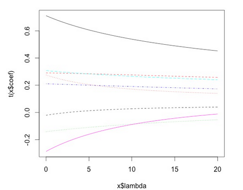
> m.ridge <- lm.ridge(lpsa ~ .,data=data.train, lambda = seq(0,20,0.1))
> plot(m.ridge)
> 
> #by using the select function
> select(m.ridge)
modified HKB estimator is 3.355691 
modified L-W estimator is 3.050708 
smallest value of GCV  at 4.9

下記のような図と共に、ベストなλは4.9だと選ばれました。

次に予測値を返させて、MSEを求めます。

> y.pred.ridge = scale(data.test[,1:8],center = m.ridge$xm, scale = m.ridge$scales)%*% m.ridge$coef[,which.min(m.ridge$GCV)] + m.ridge$ym
> summary((y.pred.ridge - y.test)^2)
       V1          
 Min.   :0.000003  
 1st Qu.:0.043863  
 Median :0.136450  
 Mean   :0.494410  
 3rd Qu.:0.443495  
 Max.   :3.809051  
> mse.ridge=sum((y.pred.ridge - y.test)^2)
> mse.ridge
[1] 14.8323

ラッソ

あまり使っている見ませんが、larsライブラリー([https://cran.r-project.org/web/packages/lars/index.html])を使います。

> library(lars)
> m.lasso <- lars(as.matrix(data.train[,1:8]),data.train$lpsa,type="lasso")
> plot(m.lasso)
> # Cross-validation
> r <- cv.lars(as.matrix(data.train[,1:8]),data.train$lpsa)
> bestfraction <- r$index[which.min(r$cv)]
> bestfraction
[1] 0.5252525

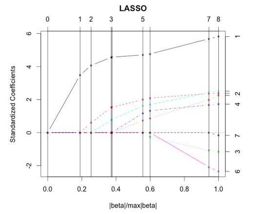
fractionは0.525あたりと図と出力から判断出来ます。

> # Observe coefficients
> coef.lasso <- predict(m.lasso,as.matrix(data.test[,1:8]),s=bestfraction,type="coefficient",mode="fraction")
> 
> # Prediction
> y.pred.lasso <- predict(m.lasso,as.matrix(data.test[,1:8]),s=bestfraction,type="fit",mode="fraction")$fit
> summary((y.pred.lasso - y.test)^2)
    Min.  1st Qu.   Median     Mean  3rd Qu.     Max. 
0.000144 0.072470 0.128000 0.454000 0.394400 3.565000 
> 
> mse.lasso=sum((y.pred.lasso - y.test)^2)
> mse.lasso
[1] 13.61874

平均二乗誤差の比較

> # Compare them 
> mse.ols
[1] 15.63822
> mse.bestsubset
[1] 15.4954
> mse.ridge
[1] 14.8323
> mse.lasso
[1] 13.61874

今回のデータに関しては、ラッソで行った分析が一番MSEを最小に出来ました。