PythonでPCAを行うにはscikit-learnを使用します。
PCAの説明は世の中に沢山あるのでここではしないでとりあえず使い方だけ説明します。
使い方は簡単です。
n_componentsはcomponentの数です。何も指定しないとデータの次元数になります。
あとは、fitにデータを渡すだけです。
from sklearn.decomposition import PCA
pca = PCA(n_components=2)
pca.fit(X)
詳細はここに書いてあります。
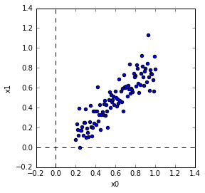
テストデータ作成
こんな感じでテスト用のデータを作成しました。
shuffleは別にしてもしなくてもどちらでもいいです。
In [10]: x = np.linspace(0.2,1,100)

In [11]: y = 0.8*x + np.random.randn(100)*0.1

In [12]: X = np.vstack([x, y]).T

In [13]: np.random.shuffle(X)
PCA
PCAは下記のようにします。
In [14]: from sklearn.decomposition import PCA

In [15]: pca = PCA(n_components=2)

In [16]: pca.fit(X)
Out[16]: PCA(copy=True, n_components=2, whiten=False)
主成分の確認
主成分はcomponents_に入っています。ついでに平均と共分散行列はmean_, get_covariance()で見れます。
In [17]: print 'components'
    ...: print pca.components_
    ...: print 'mean'
    ...: print pca.mean_
    ...: print 'covariance'
    ...: print pca.get_covariance()
    ...:
components
[[ 0.71487492  0.69925235]
 [-0.69925235  0.71487492]]
mean
[ 0.6         0.47190318]
covariance
[[ 0.05441077  0.04603365]
 [ 0.04603365  0.0523763 ]]
ここで自分で平均と共分散行列を計算してみます。
平均は各成分毎に平均したものです。
共分散行列は共分散を計算したものです。(そのまんまですが)
共分散を計算するときのbias=1は分散、共分散の分母を何にするかを指定するためのものです。
ここではデータ数で割るために1を指定しています。0だとデータ数-1で割られます。
結果が同じになっていることがわかります。
In [22]: mn = np.mean(X,axis=0)

In [23]: z = X - mn

In [24]: cv = np.cov(z[:,0],z[:,1],bias=1)

In [25]: print 'mean'
    ...: print mn
    ...: print 'covariance'
    ...: print cv
    ...:
mean
[ 0.6         0.47190318]
covariance
[[ 0.05441077  0.04603365]
 [ 0.04603365  0.0523763 ]]
次に共分散行列の固有値と固有ベクトルを計算します。
共分散行列の固有ベクトルは主成分と一致します。
固有値と固有ベクトルはnumpy.linalg.eigで計算します。
W, v = np.linalg.eig(cv)

print 'eigenvector'
print v
print 'eigenvalue'
print W

eigenvector
[[ 0.71487492 -0.69925235]
 [ 0.69925235  0.71487492]]
eigenvalue
[ 0.09943842  0.00734865]
Wが固有値でvは固有ベクトルです。
ここで、固有ベクトルは列ベクトルになっています。(縦に並んでいます)
つまりv[:,0]が第1固有ベクトルです。
components_は行ベクトル(横に並んでいます)なので注意が必要です。
一致していることがわかります。
(※たまに方向が180度反転していることがあります。)
共分散行列に固有ベクトルをかけてみます。
固有ベクトルとPCAの主成分は同じなので、共分散行列に主成分をかけていることと同じです。
固有ベクトルなので方向は変わらないです。
In [28]: print cv.dot(v[:,0].reshape(2,1))
    ...: print v[:,0]*W[0]
    ...: print cv.dot(v[:,1].reshape(2,1))
    ...: print v[:,1]*W[1]
[[ 0.07108603]
 [ 0.06953255]]
[ 0.07108603  0.06953255]
[[-0.00513856]
 [ 0.00525337]]
[-0.00513856  0.00525337]
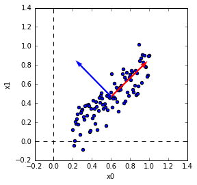
主成分ベクトルの表示
第1主成分ベクトルと第2主成分ベクトルをデータ上に表示して見ます。
第1主成分が分散の大きい方向を向いているのがわかります。
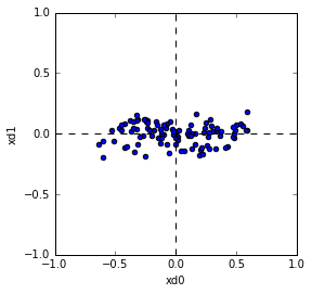
Projection
データを主成分にProjectionしてみます。
Projectionは具体的にはデータと主成分ベクトルの内積を取ることです。
In [30]: Xd = pca.transform(X)
実際にデータと主成分ベクトルの内積をとって確認してみると同じになっているのがわかります。
In [31]: print pca.components_[0]
    ...: print pca.components_[1]
    ...: print X[0,:]
    ...: print z[0,:]
    ...: print pca.components_[0].dot(z[0,:]), pca.components_[1].dot(z[0,:])
    ...: print Xd[0,:]
[ 0.71487492  0.69925235]
[-0.69925235  0.71487492]
[ 0.57979798  0.47996242]
[-0.02020202  0.00805924]
-0.00880647453855 0.0198876592146
[-0.00880647  0.01988766]
ProjectionしたデータをPlotすると下記のようになります。
Plotされた形を見ると主成分ベクトルが新しい軸になるように回転されていることがわかります。
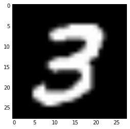
MNIST
MNISTのデータで試してみました。
MNISTは手書き文字のデータです。
データはここからダウンロードできます。
データのフォーマットもここに書いてあります。
(※今回はTensorflowのsampleコードからデータを読み込むところを拝借してきました。)
データを読み込んで、文字’3’のデータ256個を使用しました。(全部使うと多いので)
PCAは下記のようにcomponent数を50にしました。(50に特に意味はありません)
In [36]: from sklearn.decomposition import PCA

In [37]: N = 50

In [38]: pca = PCA(n_components=N)

In [39]: pca.fit(X)
Out[39]: PCA(copy=True, n_components=50, whiten=False)
主成分を画像化して表示したのが下記です。
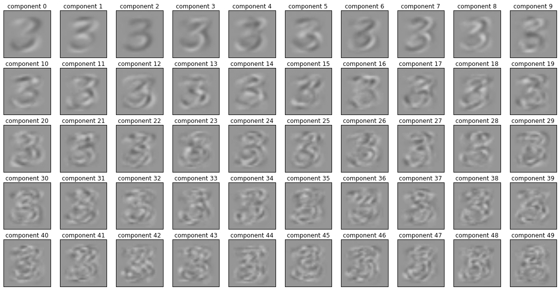
Projectionすると当然ですが50次元のデータになります。
これで次元圧縮ができます。
In [44]: Xd = pca.transform(X)

In [45]: print X.shape
(256, 784)

In [46]: print Xd.shape
(256, 50)
元の次元に戻してみます。
戻すにはinverse_transformを使用します。
In [51]: Xe = pca.inverse_transform(Xd)

In [52]: print Xe.shape
(256, 784)
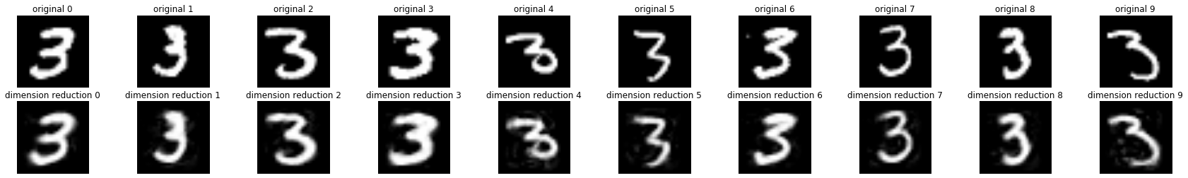
オリジナルと次元圧縮した結果を比較してみると下記のようになります。
上段がオリジナルで、下段が次元圧縮したものです。
次元数が50だったのであまり差がわかりづらいですが、微妙に違っているのがわかります。
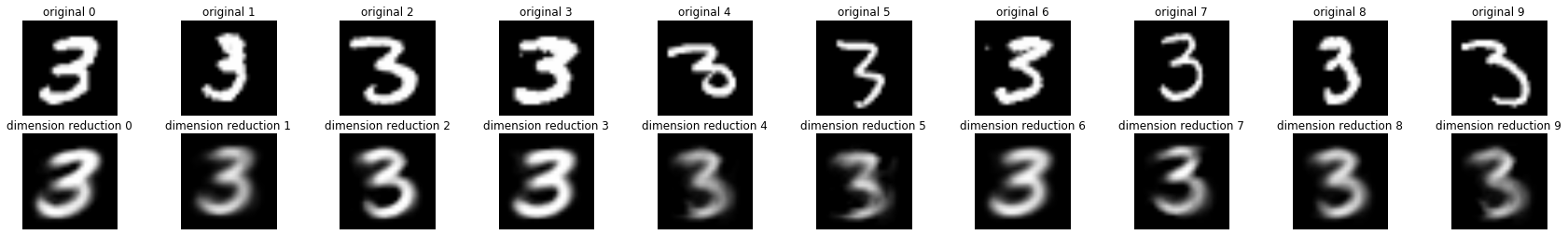
次元数を3にしてやった結果が下記になります。
次元圧縮した結果は、次元数が極端に少ないので細かい変化が表現できずにみんな同じ感じになっています。
以下使ったコードを貼りました。
code
import numpy as np
import matplotlib.pyplot as plt

# generate data
x = np.linspace(0.2,1,100)
y = 0.8*x + np.random.randn(100)*0.1
X = np.vstack([x, y]).T
np.random.shuffle(X)

# plot data
fig = plt.figure()
axes = fig.add_subplot(111,aspect='equal')
axes.scatter(X[:,0],X[:,1])
axes.set_xlim([-0.2, 1.4])
axes.set_ylim([-0.2, 1.4])
axes.set_xlabel('x0')
axes.set_ylabel('x1')
axes.vlines(0,-0.2,1.4,linestyles='dashed')
axes.hlines(0,-0.2,1.4,linestyles='dashed')

# PCA
from sklearn.decomposition import PCA
pca = PCA(n_components=2)
pca.fit(X)

# print components and mean
print 'components'
print pca.components_
print 'mean'
print pca.mean_
print 'covariance'
print pca.get_covariance()

mn = np.mean(X,axis=0)
z = X - mn
cv = np.cov(z[:,0],z[:,1],bias=1)
print 'mean'
print mn
print 'covariance'
print cv

W, v = np.linalg.eig(cv)
print 'eigenvector'
print v
print 'eigenvalue'
print W

# covariance matrix x eigenvector
print cv.dot(v[:,0].reshape(2,1))
print v[:,0]*W[0]
print cv.dot(v[:,1].reshape(2,1))
print v[:,1]*W[1]
# display
fig = plt.figure()
axes = fig.add_subplot(111,aspect='equal')
axes.scatter(X[:,0],X[:,1])
axes.set_xlim([-0.2, 1.4])
axes.set_ylim([-0.2, 1.4])
axes.set_xlabel('x0')
axes.set_ylabel('x1')
axes.vlines(0,-0.2,1.4,linestyles='dashed')
axes.hlines(0,-0.2,1.4,linestyles='dashed')
axes.quiver(pca.mean_[0], pca.mean_[1], pca.components_[0,0],pca.components_[0,1], color='red', width=0.01, scale=3)
axes.quiver(pca.mean_[0], pca.mean_[1], pca.components_[1,0],pca.components_[1,1], color='blue', width=0.01, scale=3)

# projection
Xd = pca.transform(X)
print pca.components_[0]
print pca.components_[1]
print X[0,:]
print z[0,:]
print pca.components_[0].dot(z[0,:]), pca.components_[1].dot(z[0,:])
print Xd[0,:]

fig = plt.figure()
axes = fig.add_subplot(111,aspect='equal')
axes.scatter(Xd[:,0],Xd[:,1])
axes.set_xlabel('xd0')
axes.set_ylabel('xd1')
axes.set_xlim([-1.0, 1.0])
axes.set_ylim([-1.,1.0])
axes.vlines(0,-1.0,1.0,linestyles='dashed')
axes.hlines(0,-1.0,1.0,linestyles='dashed')
# MNIST
# generate data
import numpy as np
import matplotlib.pyplot as plt
import gzip
image_filename = './data/mnist/train-images-idx3-ubyte.gz'
label_filename = './data/mnist/train-labels-idx1-ubyte.gz'
def _read32(bytestream):
  dt = np.dtype(np.uint32).newbyteorder('>')
  return np.frombuffer(bytestream.read(4), dtype=dt)[0]

with gzip.open(image_filename) as bytestream:
    magic = _read32(bytestream)
    num_images = _read32(bytestream)
    rows = _read32(bytestream)
    cols = _read32(bytestream)
    buf = bytestream.read(rows * cols * num_images)
    data = np.frombuffer(buf, dtype=np.uint8)
    data = data.reshape(num_images, rows, cols)

with gzip.open(label_filename) as bytestream:
    magic = _read32(bytestream)
    num_items = _read32(bytestream)
    buf = bytestream.read(num_items)
    labels = np.frombuffer(buf, dtype=np.uint8)

Xall = data[labels == 3, :, :]
X = Xall[0:256,:,:].reshape(256,28*28)
X = X /255.0
# PCA
from sklearn.decomposition import PCA
N = 3
pca = PCA(n_components=N)
pca.fit(X)

# plot
import matplotlib.pyplot as plt
import matplotlib.cm as cm

cols = 10
rows = int(np.ceil(N/float(cols)))

fig, axes = plt.subplots(ncols=cols, nrows=rows, figsize=(20,10))

for i in range(N):
    r = i // cols
    c = i % cols
    axes[r, c].imshow(pca.components_[i].reshape(28,28),vmin=-0.5,vmax=0.5, cmap = cm.Greys_r)
    axes[r, c].set_title('component %d' % i)
    axes[r, c].get_xaxis().set_visible(False)
    axes[r, c].get_yaxis().set_visible(False)

# projection
Xd = pca.transform(X)
print X.shape
print Xd.shape

# inverse
Xe = pca.inverse_transform(Xd)
print Xe.shape


fig, axes = plt.subplots(ncols=10, nrows=2, figsize=(30,4))


for i in range(10):
    axes[0, i].imshow(X[i,:].reshape(28,28),vmin=0.0,vmax=1.0, cmap = cm.Greys_r)
    axes[0, i].set_title('original %d' % i)
    axes[0, i].get_xaxis().set_visible(False)
    axes[0, i].get_yaxis().set_visible(False)

    axes[1, i].imshow(Xe[i,:].reshape(28,28),vmin=0.0,vmax=1.0, cmap = cm.Greys_r)
    axes[1, i].set_title('dimension reduction %d' % i)
    axes[1, i].get_xaxis().set_visible(False)
    axes[1, i].get_yaxis().set_visible(False)