はじめに
Pythonではいくつか線形回帰をするために使えるライブラリがあります。個人的に線形回帰をする必要にせまられ、そのための方法を調べたのでメモを兼ねてシェアしたいと思います。使ったライブラリは以下:
- statmodels
- scikit-learn
- PyMC3
データ準備
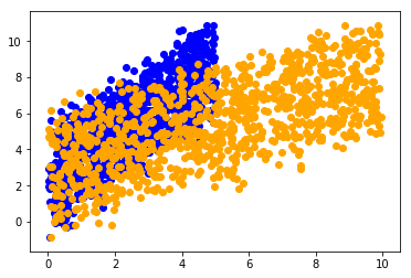
まず適当なデータを用意します。今回は以下の式にノイズ $\epsilon$ を加えた人工データを使います。
$$y = \beta_0 + \beta_1 x_1 + \beta_2 x2 + \epsilon$$
ここで推定するのは、$\beta_0, \beta_1, \beta_2$の値。
import numpy as np
import pandas as pd
import random
import matplotlib.pyplot as plt
from mpl_toolkits.mplot3d import Axes3D
# Generate random data
beta = [1.2, 0.5]
# prep data
x1 = np.random.random(size=1000)*5
x2 = np.random.random(size=1000)*10
x = np.transpose([x1, x2])
y = np.dot(x, beta) + np.random.normal(scale=0.5, size=1000)
# data = dict(x=x, y=y)
data = dict(x1=x1, x2=x2, y=y)
df = pd.DataFrame(data)
# visualisation
plt.scatter(x1, y, color='b')
plt.scatter(x2, y, color='orange')
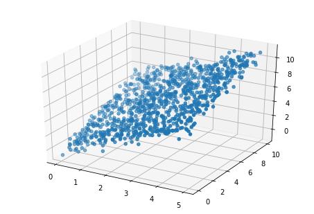
# 3D
fig = plt.figure()
ax = Axes3D(fig)
ax.scatter(x1, x2, y)
plt.show()
Statmodelsを使う場合
import statsmodels.api as sm

x = sm.add_constant(x)
results = sm.OLS(endog=y, exog=x).fit()
results.summary()
| Dep. Variable: | y | R-squared: | 0.951 |
|---|---|---|---|
| Model: | OLS | Adj. R-squared: | 0.951 |
| Method: | Least Squares | F-statistic: | 9745. |
| Date: | Fri, 10 Mar 2017 | Prob (F-statistic): | 0.00 |
| Time: | 09:58:59 | Log-Likelihood: | -724.14 |
| No. Observations: | 1000 | AIC: | 1454. |
| Df Residuals: | 997 | BIC: | 1469. |
| Df Model: | 2 | ||
| Covariance Type: | nonrobust |
| coef | std err | t | P>|t| | [95.0% Conf. Int.] | |
|---|---|---|---|---|---|
| const | 0.0499 | 0.042 | 1.181 | 0.238 | -0.033 0.133 |
| x1 | 1.1823 | 0.011 | 107.081 | 0.000 | 1.161 1.204 |
| x2 | 0.4983 | 0.005 | 91.004 | 0.000 | 0.488 0.509 |
| Omnibus: | 0.654 | Durbin-Watson: | 2.079 |
|---|---|---|---|
| Prob(Omnibus): | 0.721 | Jarque-Bera (JB): | 0.599 |
| Skew: | -0.059 | Prob(JB): | 0.741 |
| Kurtosis: | 3.023 | Cond. No. | 17.2 |
scikit-learnを使う場合
from sklearn import linear_model
# compare different regressions
lreg = linear_model.LinearRegression()
lreg.fit(x, y)
print("Linear regression: \t", lreg.coef_)
breg = linear_model.BayesianRidge()
breg.fit(x, y)
print("Bayesian regression: \t", breg.coef_)
ereg = linear_model.ElasticNetCV()
ereg.fit(x, y)
print("Elastic net:  \t\t", ereg.coef_)
print("true parameter values: \t", beta)
Linear regression: 	 [ 1.18232244  0.49832431]
Bayesian regression: 	 [ 1.18214701  0.49830501]
Elastic net:  		 [ 1.17795855  0.49756084]
true parameter values: 	 [1.2, 0.5]
PyMC3を使う場合
上2つの場合では最尤推定を使ってパラメータを推定していましたが、PyMC3ではベイズ定理に基づいてマルコフ連鎖モンテカルロ法(MCMC)でパラメータの確率分布を求めます。
import pymc3 as pm

with pm.Model() as model_robust:
    family = pm.glm.families.Normal()
    #pm.glm.glm('y ~ x', data, family=family)
    pm.glm.glm('y ~ x1+x2', df, family=family)
    start = pm.find_MAP()
    step = pm.NUTS(scaling=start)
    #step = pm.Metropolis()
    trace_robust = pm.sample(25000, step)
Optimization terminated successfully.
         Current function value: 764.008811
         Iterations: 19
         Function evaluations: 30
         Gradient evaluations: 30


100%|██████████| 25000/25000 [00:32<00:00, 761.52it/s]
# show results
pm.traceplot(trace_robust[2000:])
# pm.summary(trace_robust[2000:])
plt.show()
pm.df_summary(trace_robust[2000:])
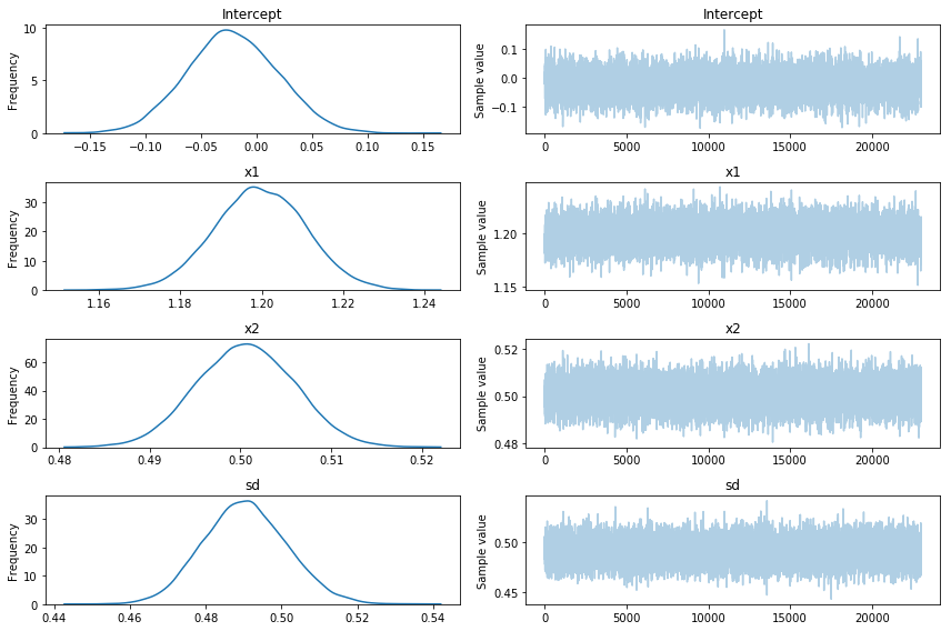
| mean | sd | mc_error | hpd_2.5 | hpd_97.5 | |
|---|---|---|---|---|---|
| Intercept | -0.022296 | 0.040946 | 0.000564 | -0.100767 | 0.057460 |
| x1 | 1.199371 | 0.011235 | 0.000126 | 1.177191 | 1.221067 |
| x2 | 0.500502 | 0.005346 | 0.000057 | 0.490258 | 0.511003 |
| sd | 0.490271 | 0.010949 | 0.000072 | 0.469599 | 0.512102 |
もうちょっと複雑な場合でやってみる
PyMC3がどこまでできるのか見るために、もうちょっと複雑な場合でやってみます。元になる式は以下:
$y = \beta_0 + \beta_1 x_1 + \beta_2 x_2+ \beta_3 x_3 + \beta_4 x_4 + \beta_5 x_5 + \epsilon$
# Generate random data
beta = [1.2, 0.5, 9.8, 0.2, 1.08]
# prep data
x1 = np.random.random(size=1000)*5
x2 = np.random.random(size=1000)*10
x3 = np.random.random(size=1000)
x4 = np.random.normal(size=1000)*2
x5 = np.random.random(size=1000)*60
x = np.transpose([x1, x2, x3, x4, x5])
y = np.dot(x, beta)  + np.random.normal(scale=0.5, size=1000)
# data = dict(x=x, y=y)
data = dict(x1=x1, x2=x2, x3=x3, x4=x4, x5=x5, y=y)
df = pd.DataFrame(data)

with pm.Model() as model_robust:
    family = pm.glm.families.Normal()
    pm.glm.glm('y ~ x1+x2+x3+x4+x5', df, family=family)
    start = pm.find_MAP()
    step = pm.NUTS(scaling=start)
    #step = pm.Metropolis()
    trace_robust = pm.sample(25000, step)
# show results
pm.traceplot(trace_robust[2000:])
plt.show()
print("true parameter values are:", beta)
pm.df_summary(trace_robust[2000:])
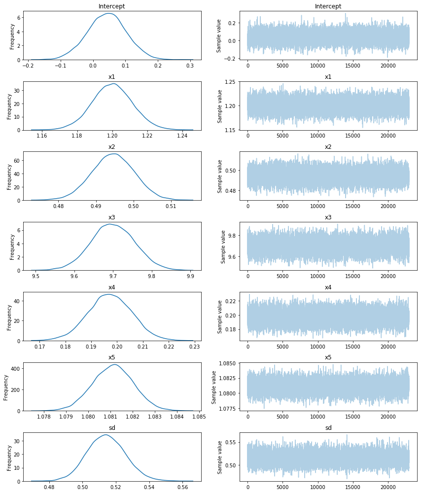
true parameter values are: [1.2, 0.5, 9.8, 0.2, 1.08]
| mean | sd | mc_error | hpd_2.5 | hpd_97.5 | |
|---|---|---|---|---|---|
| Intercept | 0.041924 | 0.059770 | 0.000737 | -0.080421 | 0.154130 |
| x1 | 1.199973 | 0.011466 | 0.000106 | 1.177061 | 1.222395 |
| x2 | 0.494488 | 0.005656 | 0.000053 | 0.483624 | 0.505661 |
| x3 | 9.699889 | 0.056527 | 0.000484 | 9.587273 | 9.809352 |
| x4 | 0.197271 | 0.008424 | 0.000052 | 0.181196 | 0.214320 |
| x5 | 1.081120 | 0.000922 | 0.000008 | 1.079339 | 1.082917 |
| sd | 0.514316 | 0.011438 | 0.000067 | 0.492296 | 0.536947 |
おわりに
短いコードで書けるので特に解説はしませんでしたが、どれもうまくパラメータを推定できていることがわかります。
もし何か質問があれば遠慮なくコメントください。
(追記) 出力画像が間違っていたので修正。