この記事は、自身のブログ、Data Science Struggleを翻訳したものになる。

概略

機械学習ライブラリを使わずにPerceptronを実装する。機械学習分野は質の良いライブラリがあり、既存のアルゴリズムを用いる分には自分で実装する必要はほとんどない。というより、自分で作ると不用意なバグが入る。
とはいえ、機械学習への理解と知識を深めるためには自分で作ってみるのも役に立つ。

なぜパーセプトロンなのか

機械学習アルゴリズムは多くの種類があるが、今回はパーセプトロンを選択。仕組みがシンプルなのと他のアルゴリズムの基礎とも言えるのが理由だ。
実際行数でいえば数十行で十分だし、必要な数学知識も線形代数くらいなものだ。実際には単純パーセプトロンくらいならわざわざ行列表記を行う必要はないが、機械学習においては線形代数の基本知識は必須なので、今回は行列計算を行う。

パーセプトロンとは何か？

パーセプトロンとはデータの入力を受け付けて、そのデータが属するクラス、ラベルの予測を返す機械学習アルゴリズムだ。もう少ししっかり書くと以下の手順を踏む。

入力を受付、重みとの線形結合を行う
上で計算された線形結合値を識別関数に渡す

以下の図がデータの流れとなる。

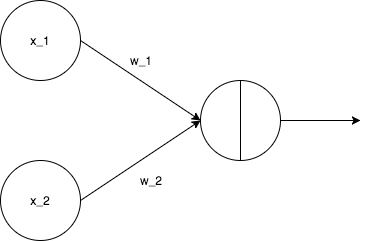
上記図のw_1、w_2を、データをうまく分けられるように更新し、定めていくことになる。

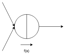
$f\left( x\right) =\begin{cases} 1,\left( x\geqq 0\right) \ -1,\left( x < 0\right) \end{cases}$

$f\left( x\right)$ above is activation function. This takes $f\left( x\right)$ as argument.

コード

import numpy as np

class Perceptron:

    def __init__(self, eta=0.1, iter_num=100):
        self.eta = eta
        self.iter_num = iter_num

    @staticmethod
    def activate(linear_combination):
        return np.where(linear_combination >= 0, 1, -1)

    def predict(self, x):
        linear_combination = np.dot(x, self.weights[1:]) + self.weights[0]
        y_pred = Perceptron.activate(linear_combination)
        return y_pred


    def fit(self, X, Y):
        self.weights = np.zeros(1 + X.shape[1])

        for _ in range(self.iter_num):
            self.error = 0
            for x, y in zip(X, Y):
                y_pred = self.predict(x)
                update = self.eta * (y - y_pred)
                self.weights[1:] += update * x
                self.weights[0] += update
                self.error += int(update != 0.0)

            print(self.error/len(Y))

        return self


from sklearn import datasets
# prepare for data
iris = datasets.load_iris()

features = iris.data
iris.target = np.where(iris.target == 0, -1, 1)

perceptron = Perceptron()
perceptron.fit(features, iris.target)

一つずつ見ていく。

def __init__(self, eta=0.1, iter_num=100):
    self.eta = eta
    self.iter_num = iter_num

init()の関数ないでetaとiter_numが初期化されている。etaはw_1、w_2の更新幅、iter_numが訓練における回数を規定する。

@staticmethod
def activate(linear_combination):
    return np.where(linear_combination >= 0, 1, -1)

ここが識別のための関数。線形結合値を入力として受付、1か-1をアウトプットする。その際、閾値は0としている。

def predict(self, x):
    linear_combination = np.dot(x, self.weights[1:]) + self.weights[0]
    y_pred = Perceptron.activate(linear_combination)
    return y_pred

この関数が予測を行うためのものになる。
linear_combinationがインプットデータと重みのドット積である。ここで、self.weights[0]だけ別に扱われているが、これはバイアス項。
y_predは予測の結果となる。

def fit(self, X, Y):
    self.weights = np.zeros(1 + X.shape[1])

    for _ in range(self.iter_num):
        self.error = 0
        for x, y in zip(X, Y):
            y_pred = self.predict(x)
            update = self.eta * (y - y_pred)
            self.weights[1:] += update * x
            self.weights[0] += update
            self.error += int(update != 0.0)

        print(self.error/len(Y))

    return self

この関数がモデルの訓練を行うためのものになる。最初の行で重みが0に初期化される。この初期化対象の重みの数はインプットデータの変数の数+1となるが、これはバイアス項の分である。

$\Delta w_{j}=n\left( y^{\left( i\right) }-\widehat {y}^{\left( i\right) }\right) x_{j}^{\left( i\right) }$

$w_{j}\leftarrow w_{j}+\Delta w_{j}$

ライブラリに頼らないパーセプトロン実装

概略

なぜパーセプトロンなのか

パーセプトロンとは何か？

コード