Python - エピデミックモデル(Kermack-McKendrick Model)のシミュレーション

エピデミック

引用：https://kotobank.jp/word/%E3%82%A8%E3%83%94%E3%83%87%E3%83%9F%E3%83%83%E3%82%AF-683127

＞エピデミック（epidemic） 医療・公衆衛生で、一定の地域や集団において、ある疾病の罹患者が、通常の予測を
＞超えて大量に発生すること。 インフルエンザなどの感染症が特定の地域で流行すること。
＞これが世界各地で同時に発生した状態をパンデミックという。

Kermack-McKendrickモデル

閉鎖集団において伝染病に感染した人の数の推移を表すモデル。
以下、連立微分方程式で表される。

\begin{eqnarray}
\frac{dx(x)}{dt}&=&-kx(t)y(t)\\
\frac{dy(t)}{dt}&=&kx(t)y(t)-ly(t)\\
\frac{dz(t)}{dt}&=&ly(t)
\end{eqnarray}

$x(t)≥0$:健康な人の数、$y(t)≥0$:病気の人の数、$z(t)≥0$:回復した人の数、$k≥0$:感染率、$l≥0$:回復率

解釈としては
・１式：
　健康な人の数$x$の変化率は、健康な人の数×病気の人の数に比例。
　比例係数が$-k$。$k,x,y≥0$なので、健康な人の数が増えることはない。
　病気の人の数が0になれば健康な人の数は一定に保たれる。
・２式：
　病気の人の数$y$の変化率は、健康な人の数の変化率と病気の人の数の寄与で決まる。
　健康な人の数の変化率が大きいor病気の人の数が多いほど病気の人の数の変化率は減少する。
　$kx(t)-l$の符号が正の場合は病気の人の数は増加し、負の場合は減少する。
・３式：
　回復した人の数$z$の変化率は、病気の人の数に比例。比例定数が$l$。病気の人が多いほど回復した人の増える速さが大きくなる。

固定点

\begin{eqnarray}
\frac{dx(x)}{dt}&=&-kx(t)y(t)=0…①\\
\frac{dy(t)}{dt}&=&kx(t)y(t)-ly(t)=0…②\\
\frac{dz(t)}{dt}&=&ly(t)=0…③
\end{eqnarray}

となる点。

②より$x$=$\frac{l}{k}$
①、③より$y=0$

保存量

\begin{eqnarray}
\frac{dx(x)}{dy(t)}&=&\frac{-kx(t)y(t)}{kx(t)y(t)-ly(t)}\\
&=&\frac{-kx(t)}{kx(t)-l}\\
(\frac{l}{k}\frac{1}{x}-1)dx(t)&=&dy(t)\\
\int{(\frac{l}{k}\frac{1}{x}-1)dx(t)}&=&\int{dy(t)}\\
\frac{l}{k}logx(t)-x(t)&=&y(t)+E
\end{eqnarray}

$\frac{l}{k}logx(t)-x(t)-y(t)$が保存量(時間が変化しても一定の値をとる)となる。

数値計算によるシミュレーション

計算方法

http://qiita.com/popondeli/items/391810fd727cefb190e7
に記載したルンゲクッタ法を連立微分方程式用に拡張して使用する。

・ソースコード

import numpy as np
import matplotlib.pyplot as plt
import math

k = 1.0
l = 1.0

DELTA_T = 0.001
MAX_T = 100.0

def dx(x, y, z, t):
    return -k * x * y

def dy(x, y, z, t):
    return k * x * y - l * y

def dz(x, y, z, t):
    return l * y

def calc_conceved_quantity(x, y, z, t):
    return (l/k)*math.log(x) - x - y

def runge_kutta(init_x, init_y, init_z, init_t):
    x, y, z, t = init_x, init_y, init_z, init_t
    history = [[x, y, z, t, calc_conceved_quantity(x, y, z, t)]]
    cnt = 0
    while t < MAX_T:
        cnt += 1
        k1_x = DELTA_T*dx(x, y, z, t)
        k1_y = DELTA_T*dy(x, y, z, t)
        k1_z = DELTA_T*dz(x, y, z, t)

        k2_x = DELTA_T*dx(x + k1_x/2, y + k1_y/2, z + k1_z/2, t + DELTA_T/2)
        k2_y = DELTA_T*dy(x + k1_x/2, y + k1_y/2, z + k1_z/2, t + DELTA_T/2)
        k2_z = DELTA_T*dz(x + k1_x/2, y + k1_y/2, z + k1_z/2, t + DELTA_T/2)

        k3_x = DELTA_T*dx(x + k2_x/2, y + k2_y/2, z + k2_z/2, t + DELTA_T/2)
        k3_y = DELTA_T*dy(x + k2_x/2, y + k2_y/2, z + k2_z/2, t + DELTA_T/2)
        k3_z = DELTA_T*dz(x + k2_x/2, y + k2_y/2, z + k2_z/2, t + DELTA_T/2)

        k4_x = DELTA_T*dx(x + k3_x, y + k3_y, z + k3_z, t + DELTA_T)
        k4_y = DELTA_T*dy(x + k3_x, y + k3_y, z + k3_z, t + DELTA_T)
        k4_z = DELTA_T*dz(x + k3_x, y + k3_y, z + k3_z, t + DELTA_T)

        x += (k1_x + 2*k2_x + 2*k3_x + k4_x)/6
        y += (k1_y + 2*k2_y + 2*k3_y + k4_y)/6
        z += (k1_z + 2*k2_z + 2*k3_z + k4_z)/6
        t += DELTA_T
        x = max(0, x)
        y = max(0, y)
        z = max(0, z)
        if cnt % 100 == 0:
            history.append([x, y, z, t, calc_conceved_quantity(x, y, z, t)])
    return history

if __name__ == '__main__':
    # ルンゲクッタ法で数値計算
    history = np.array(runge_kutta(init_x = 1, init_y = 0.1, init_z = 0, init_t = 0))

    x_min, x_max = min(history[:,0]), max(history[:,0])
    y_min, y_max = min(history[:,1]), max(history[:,1])
    z_min, z_max = min(history[:,2]), max(history[:,2])
    t_min, t_max = 0, MAX_T

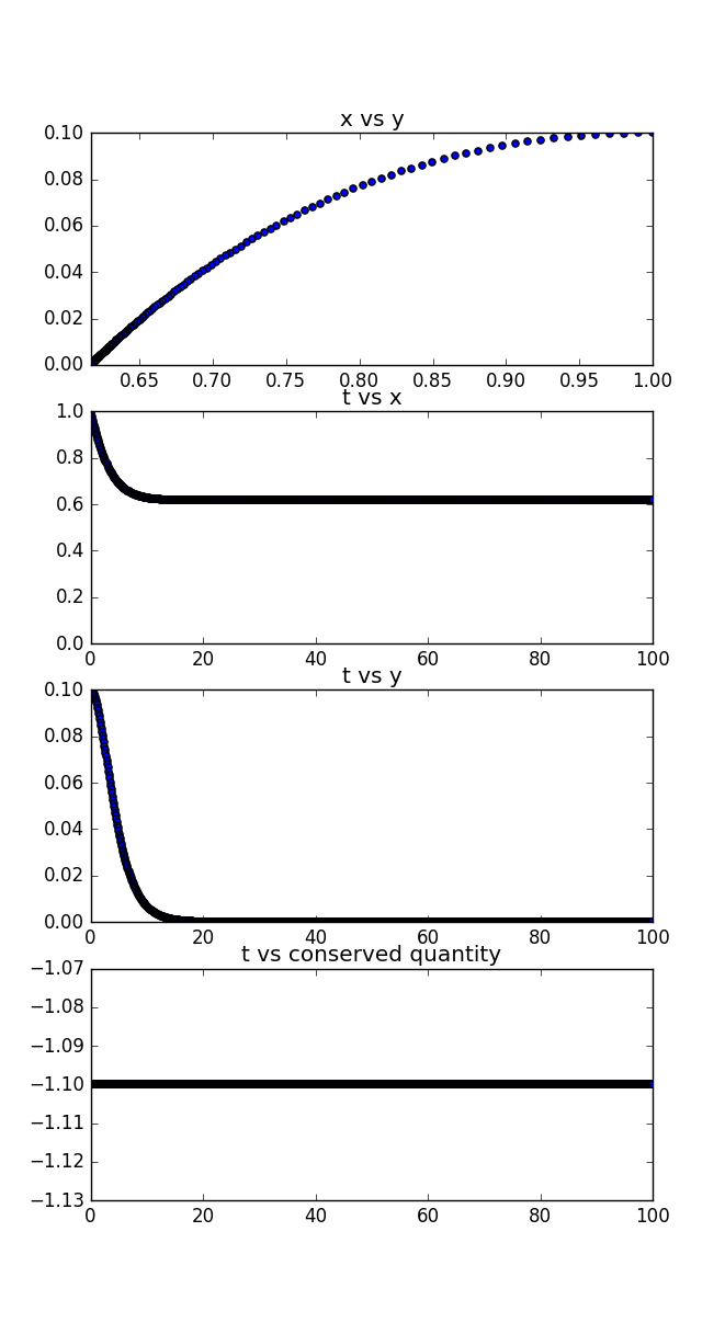
    # x vs yの位相図をプロット
    plt.subplot(4, 1, 1)
    plt.title("x vs y")
    plt.xlim(x_min, x_max)
    plt.ylim(y_min, y_max)
    plt.scatter(history[:,0], history[:,1])

    # x(健康な人の数)の時間変化をプロット
    plt.subplot(4, 1, 2)
    plt.title("t vs x")
    plt.xlim(t_min, t_max)
    plt.ylim(0, x_max)
    plt.scatter(history[:,3], history[:,0])

    # y(病気の人の数)の時間変化をプロット
    plt.subplot(4, 1, 3)
    plt.title("t vs y")
    plt.xlim(t_min, t_max)
    plt.ylim(0, y_max)
    plt.scatter(history[:,3], history[:,1])

    # 保存量の時間変化をプロット
    plt.subplot(4, 1, 4)
    plt.title(u"t vs conserved quantity")
    plt.xlim(t_min, t_max)
    plt.scatter(history[:,3], history[:,4])
    plt.show()

$k$と$l$は1.0とした。

x, y初期値の違いによる結果

$x, y$の初期値を0～1のランダムな値を与えて、100回シミュレーションを繰り返したときのx vs y位相図

ソースコード

import numpy as np
import matplotlib.pyplot as plt
import math
import random

k = 1.0
l = 1.0

DELTA_T = 0.001
MAX_T = 100.0

def dx(x, y, z, t):
    return -k * x * y

def dy(x, y, z, t):
    return k * x * y - l * y

def dz(x, y, z, t):
    return l * y

def calc_conceved_quantity(x, y, z, t):
    return (l/k)*math.log(x) - x - y

def runge_kutta(init_x, init_y, init_z, init_t):
    x, y, z, t = init_x, init_y, init_z, init_t
    history = [[x, y, z, t, calc_conceved_quantity(x, y, z, t)]]
    cnt = 0
    while t < MAX_T:
        cnt += 1
        k1_x = DELTA_T*dx(x, y, z, t)
        k1_y = DELTA_T*dy(x, y, z, t)
        k1_z = DELTA_T*dz(x, y, z, t)

        k2_x = DELTA_T*dx(x + k1_x/2, y + k1_y/2, z + k1_z/2, t + DELTA_T/2)
        k2_y = DELTA_T*dy(x + k1_x/2, y + k1_y/2, z + k1_z/2, t + DELTA_T/2)
        k2_z = DELTA_T*dz(x + k1_x/2, y + k1_y/2, z + k1_z/2, t + DELTA_T/2)

        k3_x = DELTA_T*dx(x + k2_x/2, y + k2_y/2, z + k2_z/2, t + DELTA_T/2)
        k3_y = DELTA_T*dy(x + k2_x/2, y + k2_y/2, z + k2_z/2, t + DELTA_T/2)
        k3_z = DELTA_T*dz(x + k2_x/2, y + k2_y/2, z + k2_z/2, t + DELTA_T/2)

        k4_x = DELTA_T*dx(x + k3_x, y + k3_y, z + k3_z, t + DELTA_T)
        k4_y = DELTA_T*dy(x + k3_x, y + k3_y, z + k3_z, t + DELTA_T)
        k4_z = DELTA_T*dz(x + k3_x, y + k3_y, z + k3_z, t + DELTA_T)

        x += (k1_x + 2*k2_x + 2*k3_x + k4_x)/6
        y += (k1_y + 2*k2_y + 2*k3_y + k4_y)/6
        z += (k1_z + 2*k2_z + 2*k3_z + k4_z)/6
        t += DELTA_T
        x = max(0, x)
        y = max(0, y)
        z = max(0, z)
        if cnt % 100 == 0:
            history.append([x, y, z, t, calc_conceved_quantity(x, y, z, t)])
    return history

if __name__ == '__main__':

    for i in range(0, 100):
        init_x = random.random()
        init_y = random.random()

        # ルンゲクッタ法で数値計算
        history = np.array(runge_kutta(init_x, init_y, init_z = 0, init_t = 0))

        x_min, x_max = min(history[:,0]), max(history[:,0])
        y_min, y_max = min(history[:,1]), max(history[:,1])
        z_min, z_max = min(history[:,2]), max(history[:,2])
        t_min, t_max = 0, MAX_T

        # x vs yの位相図をプロット
        plt.title("x vs y")
        plt.xlim(0, 1)
        plt.ylim(0, 1)
        plt.scatter(history[:,0], history[:,1])
    plt.show()

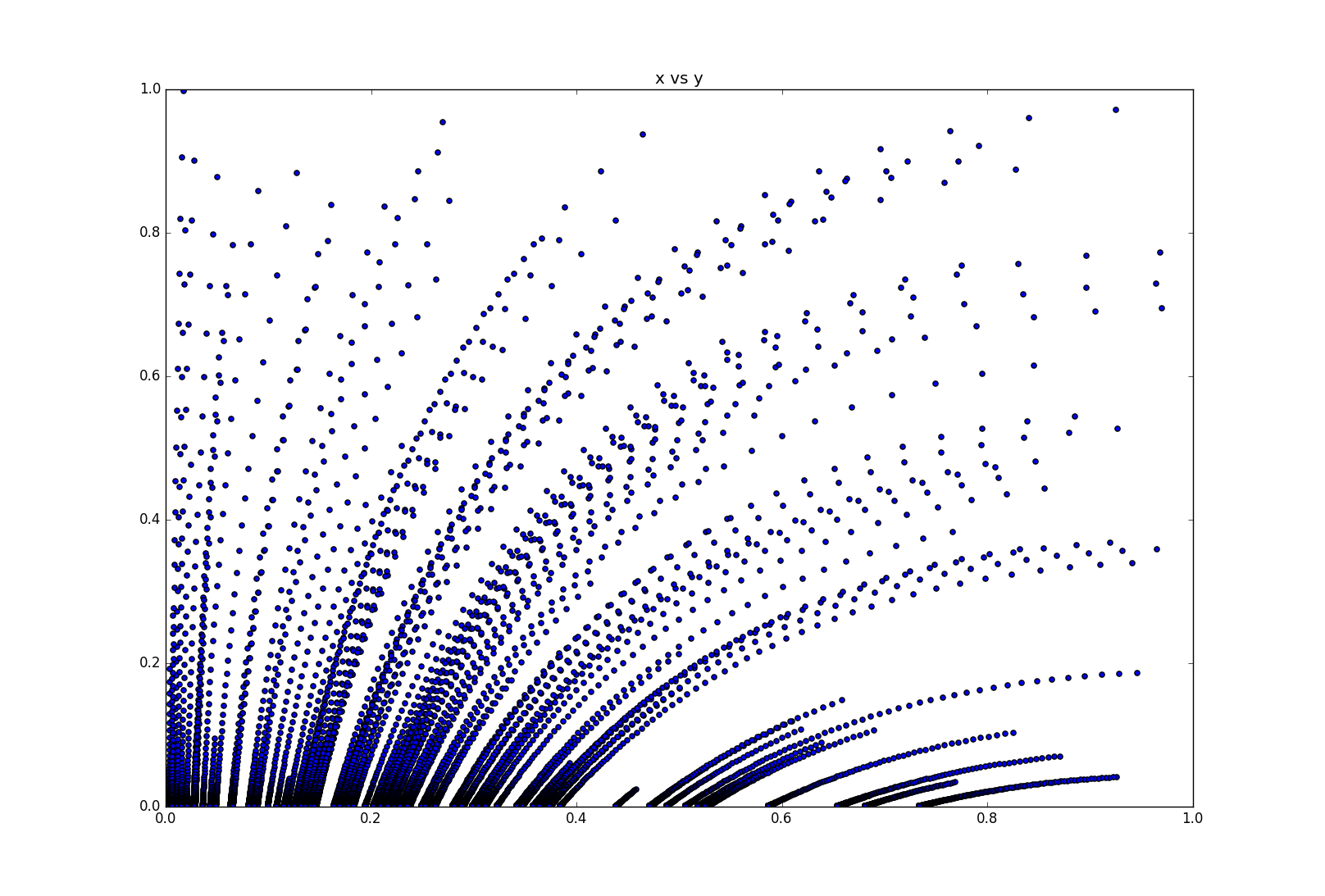
カーブを描きながら$y=0$(=感染者数0)へ落ちていく。

パラメータk,l(感染率、回復率)の違いによる結果

回復率高め

$l = 3.0$、$k = 1.0$

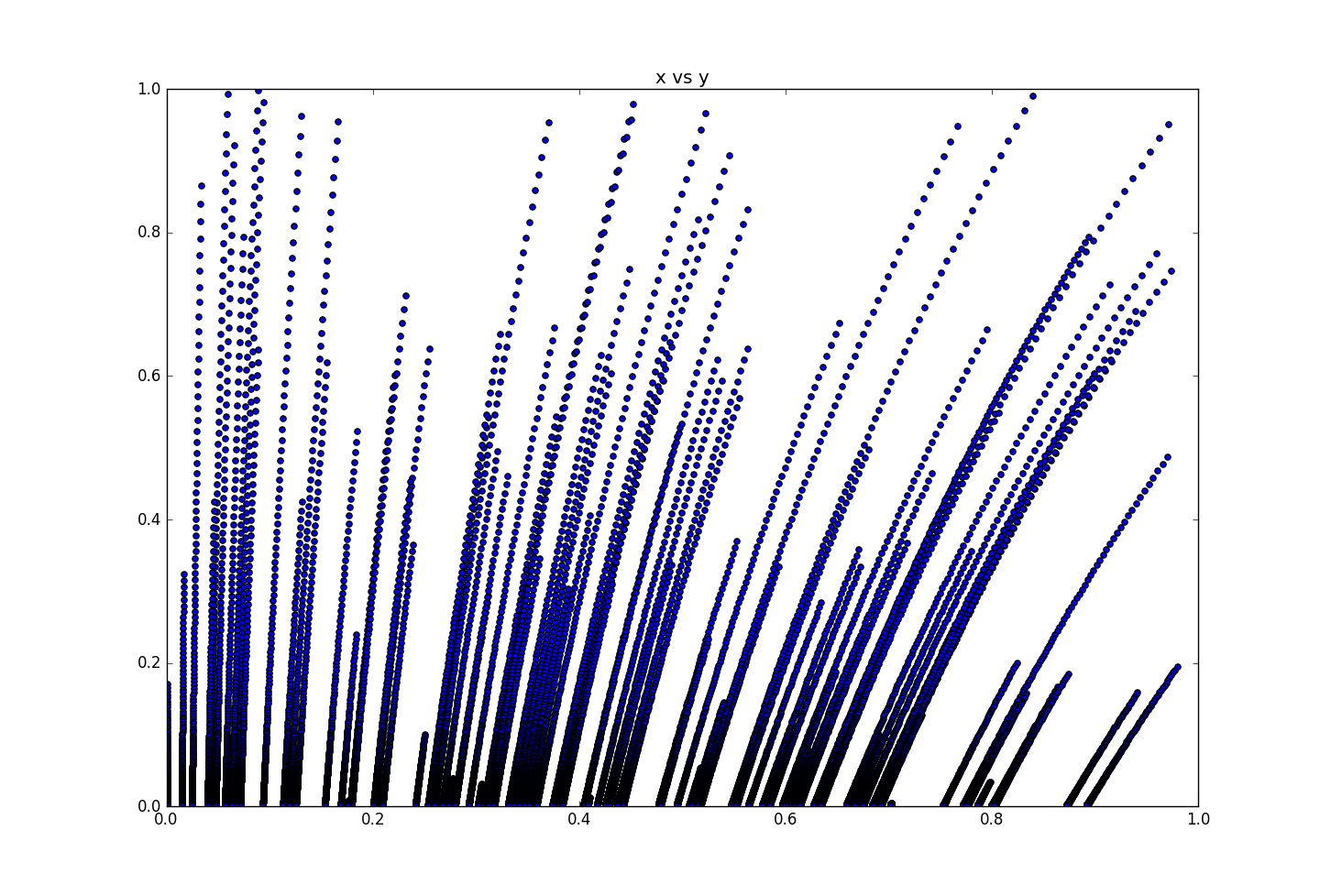
$y = 0$への落ち方が急になる

感染率高め

$l = 1.0$、$k = 5.0$

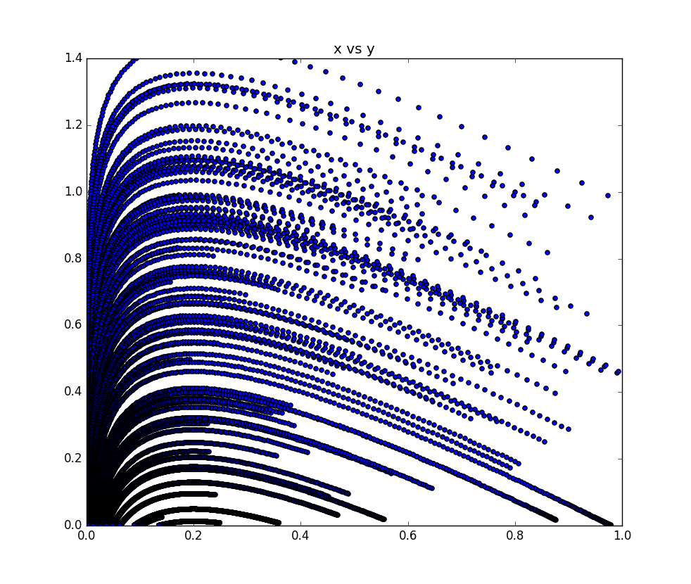
一度感染者は増え0へと減少していく