背景
Rを使う人たちは、回帰をすることが多いと思います。それにも関わらず、RのMXnetの回帰に関する資料は、日本語、英語を問わず、とても少ない気がします。公式のチュートリアルにも最低限の例しかのっていません(RとMXnetを組み合わせるというのが、Deep learningの選択肢として正しくないのかも?)。そこで、簡単な例題を通じて、RのMXnetの回帰を使ってみたいと思います。
今回あつかうデータは、Sinカーブに正規分布ノイズを加えたデータものです。これをRのMXNetでフィットさせてみることを目標としました。
(本ページは初心者が書いてるので、誤りを含むかもしれません)

データ
以下のように、未知の非線形関数f(x)(実際はsin)に平均0で標準偏差0.5で正規分布するノイズを加えたものを、データとして考えます。
y = f(x) + \epsilon\\

\epsilon \sim Normal(0, 0.5)
set.seed(1)
n_sample <- 100
xx <- seq(-5, 5, length = n_sample)
mu <- 2 + sin(xx)
yy <- rnorm(n_sample, mu, 0.5)
モデルを作る
Deep learningのモデルを作っていきます。中間層は3層で、ノードの数はBaysian Optimizationにより決めした。この記事などが参考にります。
library(mxnet)

data <- mx.symbol.Variable("data")

fc1 <- mx.symbol.FullyConnected(data, name = "fc1", num_hidden = 100)
act1 <- mx.symbol.Activation(fc1, name = "relu1", act_type = "relu")
drop1 <- mx.symbol.Dropout(act1, p = 0.2)

fc2 <- mx.symbol.FullyConnected(act1, name = "fc2", num_hidden = 49)
act2 <- mx.symbol.Activation(fc2, name = "relu2", act_type = "relu")
drop2 <- mx.symbol.Dropout(act2, p = 0.2)

fc3 <- mx.symbol.FullyConnected(drop2, name = "fc3", num_hidden = 53)
act3 <- mx.symbol.Activation(fc3, name = "relu3", act_type = "relu")
drop3 <- mx.symbol.Dropout(act3, p = 0.2)

fc4 <- mx.symbol.FullyConnected(drop3, num_hidden = 1)

output <- mx.symbol.LinearRegressionOutput(fc4)
パラメータを学習させる1
パラメータを学習させていきます。Learning rateもBaysian Optimizationで得られた値を使っています。予測力の高いモデルを作るためには、本来はtrainとtestのデータを分けるべきですが、今回は簡易化のために、フィットさせるところまでを目的としてるので、全データをまとめて使っています。またデータは正規化させず、そのままの値を使っています。
mx.set.seed(1)

model <- mx.model.FeedForward.create(output, X = xx, y = yy,
                                       ctx = mx.cpu(),
                                       num.round = 124,
                                       array.batch.size = 100,
                                       initializer = mx.init.uniform(0.01),
                                       learning.rate = 0.0789,
                                       momentum = 0.9,
                                       eval.metric = mx.metric.rmse)

Start training with 1 devices
[1] Train-rmse=NaN
[2] Train-rmse=2.23326795346586
[3] Train-rmse=2.08504108125293
[4] Train-rmse=1.82124038961198
[5] Train-rmse=1.48954090785246
[6] Train-rmse=1.15752385720034
[7] Train-rmse=0.923669173895963
# ...#

[123] Train-rmse=0.875656856417879
[124] Train-rmse=0.875656267602696
学習するごとに、RMSEは小さくなっていますが、実は全く上手くいっていません。下の図のようにlocal minima(この場合、yの平均値)に引っかかっています。他のデータで試しても、同じような失敗をすることが多いようです。

ここで、一番のポイントは、initializerの値です。デフォルトでは、initializer = mx.init.uniform(0.01)となっていますが、ここを少し変更する必要があります。
パラメータを学習させる2
initializer = mx.init.uniform(0.2)と変更して、再チャレンジします。Baysian Optimizationも、mx.init.uniform(0.2)を使っています。これで、初期値を$uniform(-0.2, 0.2)$から、とってくるということになります。
model <- mx.model.FeedForward.create(output, X = xx, y = yy,
                                       ctx = mx.cpu(),
                                       num.round = 124,
                                       array.batch.size = 100,
                                       initializer=mx.init.uniform(0.2),
                                       learning.rate = 0.0789,
                                       momentum = 0.9,
                                       eval.metric=mx.metric.rmse)

Start training with 1 devices
[1] Train-rmse=NaN
[2] Train-rmse=2.12165792635148
[3] Train-rmse=1.65953289558761
[4] Train-rmse=1.1639932568447
[5] Train-rmse=1.53508849050074
[6] Train-rmse=1.45345311053074
[7] Train-rmse=0.977683196174199
# ...#
[123] Train-rmse=0.467904513556867
[124] Train-rmse=0.443160963247551
今度は、local minimaに引っかかることなく、それなりに上手くフィットさせることができました。予測のラインは、$x > 3\pi/2$のあたりでも減少関数になってしまっていますが、このデータからは、これが限界かと思われます。

学習していく様子
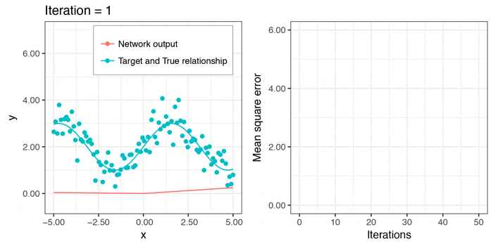
せっかくなので、学習していく様子のgifも作ってみました。
まとめ
調整しないといけないパラメータが多いです。また、初期値を決める確率分布に関する説明があまり見当たらなかったので、ここを設定しなくてはいけないことに気づくのに、かなり時間がかかりました。とりあえず、RでもDeep learningで回帰ができそうです。
環境
sessionInfo()
R version 3.3.2 (2016-10-31)
Platform: x86_64-pc-[uploading-0](...)
linux-gnu (64-bit)
Running under: Ubuntu 14.04.5 LTS
参考
- A Gentle Introduction to Artificial Neural Networks
- Deep Learning 入門(2) - Chainerで自作の非線形回帰を試そう -
- Develop a Neural Network with MXNet in Five Minutes
- [Deep Learningで遊ぶ(2): オンラインニュース人気度+ベイズ最適化によるパラメータチューニング] (http://tjo.hatenablog.com/entry/2016/07/21/190000)
おまけ:全体のコード
library(mxnet)
library(rBayesianOptimization)
library(dplyr)
library(Metrics)
library(ggplot2)
library(cowplot)

# データの準備
set.seed(1)
n_sample <- 100
xx <- seq(-5, 5, length = n_sample)
mu <- 2 + sin(xx)
yy <- rnorm(n_sample, mu, 0.5)


# Bayesian Optimization
mxnet_holdout_bayes <- function(unit1, unit2, unit3, num_r, learn_r){
     data <- mx.symbol.Variable("data")
     fc1 <- mx.symbol.FullyConnected(data, name="fc1", num_hidden=unit1)
     act1 <- mx.symbol.Activation(fc1, name="relu1", act_type="relu")
     drop1 <- mx.symbol.Dropout(act1, p=0.2)
     fc2 <- mx.symbol.FullyConnected(drop1, name="fc2", num_hidden=unit2)
     act2 <- mx.symbol.Activation(fc2, name="relu2", act_type="relu")
     drop2 <- mx.symbol.Dropout(act2, p=0.2)
     fc3 <- mx.symbol.FullyConnected(drop2, name="fc3", num_hidden=unit3)
     act3 <- mx.symbol.Activation(fc3, name="relu3", act_type="relu")
     drop3 <- mx.symbol.Dropout(act3, p=0.2)
     fc4 <- mx.symbol.FullyConnected(drop3, name="fc4", num_hidden=1)
     output <- mx.symbol.LinearRegressionOutput(fc4, name="linreg")
     devices <- mx.cpu()

     mx.set.seed(1)
     model <- mx.model.FeedForward.create(output, X=xx,
      y=yy,
       ctx=devices, num.round=num_r, array.batch.size=100,
       learning.rate=learn_r, momentum=0.9,
       eval.metric=mx.metric.rmse,
       initializer=mx.init.uniform(0.2),
       epoch.end.callback=mx.callback.log.train.metric(20),
      verbose=FALSE)

     preds <- predict(model, data.matrix(xx), array.layout='rowmajor')
     holdout_score <- rmse(preds, yy)
     list(Score=-holdout_score, Pred=-holdout_score)
 }

# Bayesian Optimizationの実行
opt_res <- BayesianOptimization(mxnet_holdout_bayes,
                               bounds=list(unit1=c(1L,100L),
                                           unit2=c(1L,100L),
                                           unit3=c(1L,100L),
                                           num_r=c(10L,150L),
                                           learn_r=c(1e-5,1e-1)),
                               init_points=50, n_iter=1, acq='ucb', kappa=2.576, eps=0.0, verbose=TRUE)
# Best Parameters Found:
# Round = 51      unit1 = 100.0000        unit2 = 49.0000 unit3 = 53.0000 num_r = 124.0000        learn_r = 0
# .0789   Value = -0.4390

# モデル
data <- mx.symbol.Variable("data")
fc1 <- mx.symbol.FullyConnected(data, name="fc1",
 num_hidden=opt_res$Best_Par[1]))
act1 <- mx.symbol.Activation(fc1, name="relu1", act_type="relu")
drop1 <- mx.symbol.Dropout(act1, p=0.2)
fc2 <- mx.symbol.FullyConnected(drop1, name="fc2",
 num_hidden=opt_res$Best_Par[2]))
act2 <- mx.symbol.Activation(fc2, name="relu2", act_type="relu")
drop2 <- mx.symbol.Dropout(act2, p=0.2)
fc3 <- mx.symbol.FullyConnected(drop2, name="fc3",
 num_hidden=opt_res$Best_Par[3])
act3 <- mx.symbol.Activation(fc3, name="relu3", act_type="relu")
drop3 <- mx.symbol.Dropout(act3, p=0.2)
fc4 <- mx.symbol.FullyConnected(drop2, name="fc4", num_hidden=1)
output <- mx.symbol.LinearRegressionOutput(fc4, name="linreg")


# ggplotでのメモリ調整用関数
fmt_dcimals <- function(x) format(x, nsmall = 2, scientific = FALSE)

# 成功一枚分の作図
pdf("good.pdf", width = 3.5, height = 3.5)
  mx.set.seed(1)
  model <- mx.model.FeedForward.create(output, X=xx, y=yy,
                                         ctx=mx.cpu(),
                                         num.round=opt_res$Best_Par[4],
                                         array.batch.size=100,
                                         initializer=mx.init.uniform(0.2),
                                         learning.rate=opt_res$Best_Par[5],
                                         momentum=0.9,
                                         eval.metric=mx.metric.rmse)

   preds <-  predict(model, data.matrix(xx))

  fig_dat <- data_frame(xx, yy, mu, preds = preds[1,]) %>%
   tidyr::gather(cat, val, 2:4) %>%
   mutate(cat = factor(cat, levels = c("mu", "yy", "preds"))) %>%
   mutate(cat = factor(cat, labels = c("True relationship", "Target", "Network output"))) %>%
   mutate(cat2 = ifelse(cat == "Network output", "Network output", "Target and True relationship") %>% as.factor)

  p1 <- ggplot(fig_dat %>% arrange(val), aes(x = xx, y = val)) +
   geom_point(data = fig_dat %>% filter(cat == "Target"), aes(colour = cat2)) +
   geom_line(data = fig_dat %>% filter(cat != "Target"), aes(colour = cat2)) +
   guides(colour = guide_legend(title = NULL,
   order = 1)) +
   labs(x = "x", y = "y") +
   theme_bw() +
   theme(legend.position = c(0.6, 0.85),
         legend.background = element_rect(colour = "black",
           linetype = "solid", size = 0.1)) +
   scale_y_continuous(limits = c(-0.5, 7), labels=fmt_dcimals)
  p1
dev.off()


# 130枚分の作図
mse_v <- NULL
n <- 3
hues <- seq(15, 375, length=n+1)
cols_hex <- sort(hcl(h=hues, l=65, c=100)[1:n])

for (i in 1:130){
  mx.set.seed(1)
  model <- mx.model.FeedForward.create(output, X=xx, y=yy,
                                         ctx=mx.cpu(),
                                         num.round=i,
                                         array.batch.size=100,
                                         initializer=mx.init.uniform(0.2),
                                         learning.rate=0.0789,
                                         momentum=0.9,
                                         eval.metric=mx.metric.rmse)

   preds <-  predict(model, data.matrix(xx))
   mse_v[i] <- (preds - yy)^2 %>% mean

   if (i < 10) i2 <- paste("00", i, sep = "")  else if (i < 100) i2 <- paste(0, i, sep = "") else i2 <- i
   pdf(paste(i2, "_fig.pdf", sep = ""), width = 7, height = 3.5)
   fig_dat <- data_frame(xx, yy, mu, preds = preds[1,]) %>%
    tidyr::gather(cat, val, 2:4) %>%
    mutate(cat = factor(cat, levels = c("mu", "yy", "preds"))) %>%
    mutate(cat = factor(cat, labels = c("True relationship", "Target", "Network output"))) %>%
    mutate(cat2 = ifelse(cat == "Network output", "Network output", "Target and True relationship") %>% as.factor)

   p1 <- ggplot(fig_dat %>% arrange(val), aes(x = xx, y = val)) +
    geom_point(data = fig_dat %>% filter(cat == "Target"), aes(colour = cat2)) +
    geom_line(data = fig_dat %>% filter(cat != "Target"), aes(colour = cat2)) +
    guides(colour = guide_legend(title = NULL,
    order = 1)) +
    labs(title = paste("Iteration =", i), x = "x", y = "y") +
    theme_bw() +
    theme(legend.position = c(0.6, 0.85),
          legend.background = element_rect(colour = "black",
            linetype = "solid", size = 0.1)) +
    scale_y_continuous(limits = c(-0.5, 7), labels=fmt_dcimals) +
    scale_x_continuous(labels=fmt_dcimals)


    if (i != 1) fig_dat2 <- data_frame(MSE = mse_v, Iteration = 1:i) else fig_dat2 <- data_frame(MSE = 0, Iteration = 1:i)

    if (i < 20) ylim_max <- 6 else if (i < 50) ylim_max <- 2 else if (i < 75) ylim_max <- 1 else ylim_max <- 0.5
    if (i < 20) xlim_max <- 50 else  if (i < 80) xlim_max <- 100 else xlim_max <- 130

    p2 <- ggplot(fig_dat2, aes(x = Iteration, y = MSE)) +
      geom_path(colour = cols_hex[2]) +
      labs(title = "", x = "Iterations", y = "Mean square error") +
      xlim(0, xlim_max) +
      theme_bw() +
      scale_y_continuous(limits = c(0, ylim_max), labels=fmt_dcimals)

    p3 <- plot_grid(p1, p2, align = "hv")
    print(p3)

   dev.off()
}