{rstan} 欠損値あり時系列データのモデル推定

サンプルデータ

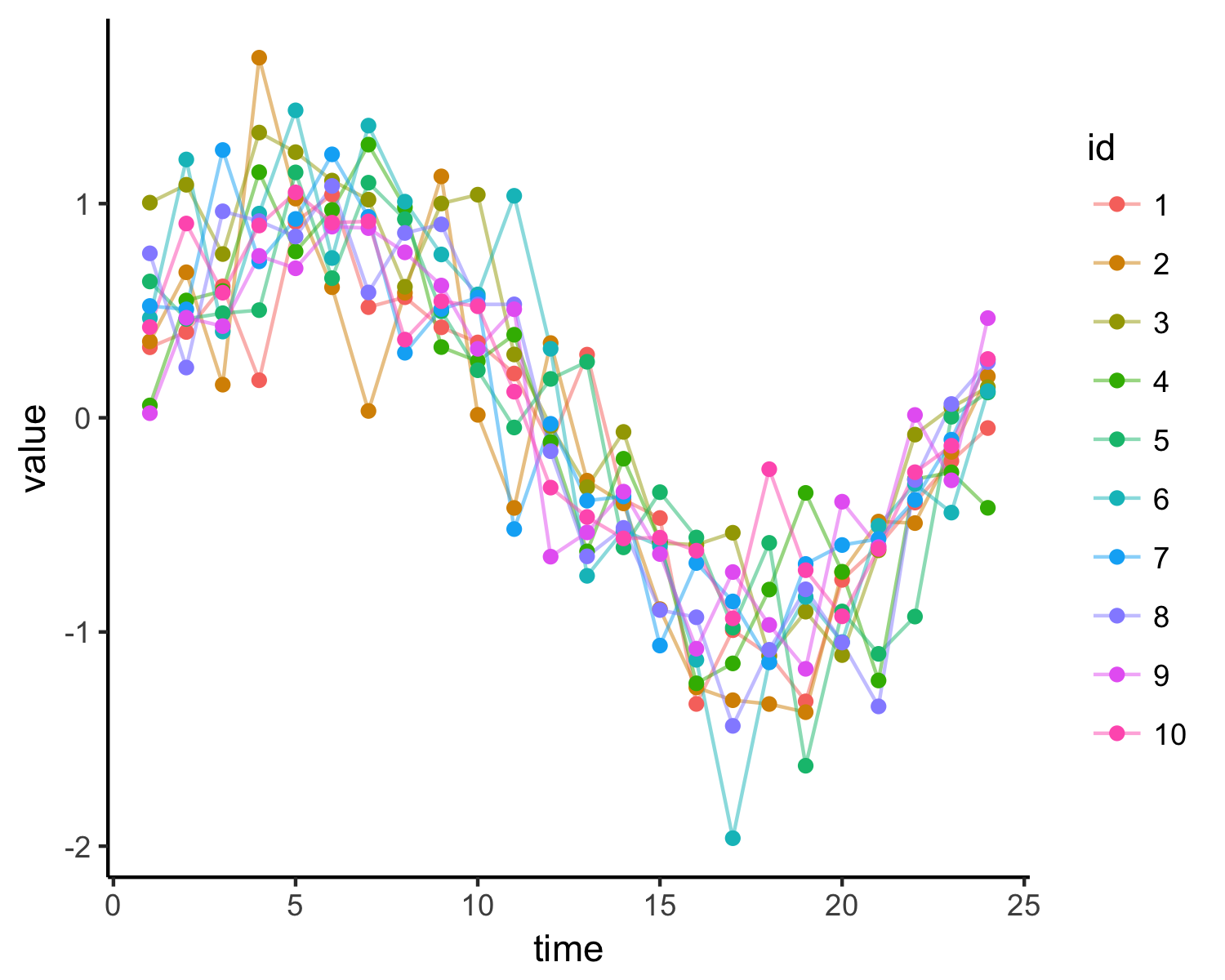
適当なサンプルデータを用意します。

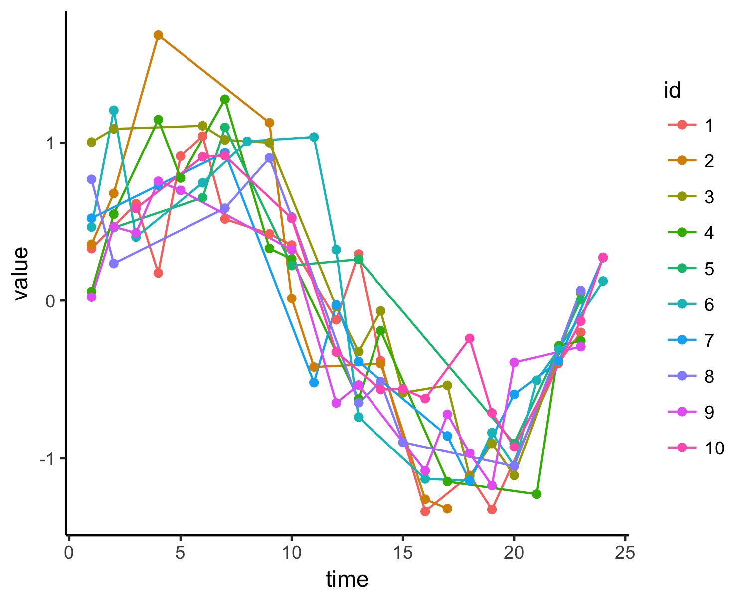
ランダムにデータの半分をブッコヌキます。

モデル

神様の方法を真似して、2階差分を仮定します。

\begin{eqnarray}
&\mu_t - \mu_{t-1} &\sim& normal(\mu_{t-1} - \mu_{t-2},\ s_{mu})\\
\leftrightarrow &\mu_t &\sim& normal(2*\mu_{t-1} - \mu_{t-2},\ s_{mu})
\end{eqnarray}

stan code

えーと、方法は2つあります。

・個々のIDごとの補完を行いたい場合
　　→ 　神の書の9.5.2 欠測値を参照。
・全体の傾向を抽出したい場合
　　→ 大元のマニュアルのChapter 15を参照。

ここでは後者。
まんまなので、コードを載せて終わらせますが、$segment$を使うのがポイントです。

系列idごとのtimeが揃っていないという困難を回避する為の細工です。
これは、いわゆる「縦長データ」(R業界ではtidyなデータと呼びますが)を作っておいて、グループごとのサンプルサイズ(変数Sに格納)と共に処理するものです。

データYはベクトルで与えられ、Sに従って1:N_timeに分解されるという理屈です。

  data{
    int N_sample;
    int N_time;

    vector[N_sample] Y;
    int S[N_time];
  }

  parameters{
    real<lower = 0> s;
    real<lower = 0> s_mu;
    real mu[N_time];
  }

  model{
    int pos;
    pos = 1;
    for(k in 1:N_time){
      segment(Y, pos, S[k]) ~ normal(mu[k], s);
      pos = pos + S[k];
    }

    for(k in 3:N_time){
      mu[k] ~ normal(2 * mu[k-1] - mu[k-2], s_mu);
    }
  }

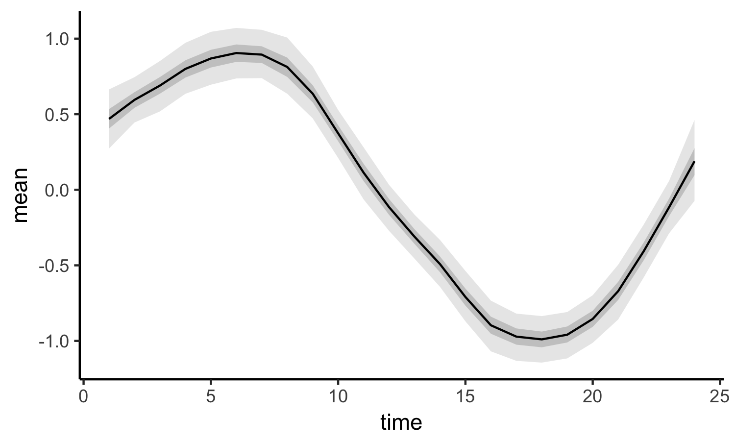
結果

Appendix

サンプルデータ

set.seed(111)

N_time <- 24
N_id <- 10
SD <- 0.3

x <- 1:N_time
y <- sin(x/N_time * 2 * pi)

dat <- data.frame(time = x, id = factor(rep(1:N_id, each = N_time)),
                  value = rnorm(N_time * N_id, y, SD))

# 一様乱数を使ってデータを半分にしています。
dat1 <- dat %>% 
  dplyr::mutate(index = runif(N_time * N_id, 0, 1)) %>% 
  dplyr::filter(index > 0.5)

stan キックコード

datastan <- list(N_sample = nrow(dat1), N_time = N_time,
                 Y = dat1$value[order(dat1$time)], 
                 S = as.numeric(table(dat1$time)))

# stanコードはテキストにしてstanmodelという変数に格納しておきます。
fit <- stan(model_code = stanmodel, data = datastan, seed = 123)

お絵かき

サンプルデータの図

ggplot(dat, aes(time, value))+
  theme_classic()+
  geom_path(aes(color = id), alpha = 0.5)+
  geom_point(aes(color = id))

stan の結果の図

色々な描き方があるので、お好みで。

dat_g <- tidy(summary(fit)$summary) %>% 
  filter(.rownames %in% paste("mu[", 1:N_time, "]", sep = "")) %>% 
  mutate(time = as.numeric(str_sub(.rownames, start = 4, end = -2)))


ggplot(dat_g, aes(x = time, y = mean))+
  theme_classic()+
  geom_ribbon(aes(ymax = X97.5., ymin = X2.5.), fill = "lightgrey", alpha =0.5)+
  geom_ribbon(aes(ymax = X75., ymin = X25.), fill = "darkgrey", alpha =0.5)+
  geom_line()

環境

> sessionInfo()
R version 3.3.1 (2016-06-21)
Platform: x86_64-apple-darwin13.4.0 (64-bit)
Running under: OS X 10.10.5 (Yosemite)

attached base packages:
[1] stats     graphics  grDevices utils     datasets  methods   base     

other attached packages:
[1] stringr_1.2.0        broom_0.4.1          ggmcmc_1.1          
[4] tidyr_0.6.0          rstan_2.14.1         StanHeaders_2.14.0-1
[7] ggplot2_2.2.1        dplyr_0.5.0