※ 自分用
つらつらと自分用のPython Tipsが並ぶだけで説明はありません。
随時更新で徐々に充実させていく用途です。
from __future__ import division, unicode_literals
一般
# リストの要素毎に数を数える
from collections import defaultdict
cnt_dict = defaultdict(int)

data = x = np.random.randint(low=0, high=5, size=500)
for d in data:
    cnt_dict[d] += 1

print cnt_dict
out
defaultdict(<type 'int'>, {0: 90, 1: 113, 2: 94, 3: 96, 4: 107})
- 利用ライブラリのバージョンチェックと不適合の場合のアサート
# ライブラリのバージョンチェック
from distutils.version import LooseVersion

# 使用例
assert LooseVersion(tf.__version__) >= LooseVersion("1.3")
# もっと便利なカウントの仕方
import  numpy as np
from collections import Counter

data1 = np.random.randint(low=0, high=5, size=300)
cnt1 = Counter(data1)
print cnt1

data2 = np.random.randint(low=0, high=10, size=500)
cnt2 = Counter(data2)
print cnt2

print cnt1 + cnt2
out
Counter({3: 65, 0: 64, 1: 60, 4: 60, 2: 51})
Counter({4: 58, 8: 58, 1: 55, 6: 54, 0: 53, 2: 49, 3: 47, 5: 46, 7: 40, 9: 40})
Counter({4: 118, 0: 117, 1: 115, 3: 112, 2: 100, 8: 58, 6: 54, 5: 46, 7: 40, 9: 40})
# Pickleする
import cPickle as pickle
def unpickle(filename):
    with open(filename, 'rb') as fo:
        _dict = pickle.load(fo)
    return _dict

def to_pickle(filename, obj):
    with open(filename, 'wb') as f:
        pickle.dump(obj, f, -1)
        # pickle.Pickler(f, 2).dump(obj)
# webページからリンクの抽出
from bs4 import BeautifulSoup
import requests
from requests_oauthlib import OAuth1Session

url = 'http://headlines.yahoo.co.jp/rss/list'
url_list = []
res = requests.get(url)
news_all = BeautifulSoup(res.text, "xml")
for link in news_all.find_all('a'):
    url = link.get('href')
    print url
h5でsave&load
import deepdish as dd

dd.io.save("../data/df_test.h5", df_test)
df_test = dd.io.load("../data/df_test.h5")
# 小数点第何位まで表示するか
%precision 4
np.pi
out
3.1416
描画関連
# 定型インポート文
%matplotlib inline
import matplotlib.pyplot as plt
import numpy as np
import pandas as pd
from datetime import diatomite as dt
import sys
plt.style.use('ggplot')

# Texを使う時
plt.rc('text', usetex=True)
plt.rc('font', family='serif')
Pandas Dataframe
数字に見える文字列を、数値型に変換する
# http://stackoverflow.com/questions/21197774/assign-pandas-dataframe-column-dtypes

In [11]: df
Out[11]:
   x  y
0  a  1
1  b  2

In [12]: df.dtypes
Out[12]:
x    object
y    object
dtype: object

In [13]: df.convert_objects(convert_numeric=True)
Out[13]:
   x  y
0  a  1
1  b  2

In [14]: df.convert_objects(convert_numeric=True).dtypes
Out[14]:
x    object
y     int64
dtype: object
# カテゴリ変数(Rで言うfactory型)的な扱いについて
%matplotlib inline
from matplotlib import pyplot as plt
import numpy as np
import pandas as pd
import seaborn as sns
sns.set()

df = sns.load_dataset("tips")
for c in ['sex', 'smoker', 'day', 'time',]:
    df["c{}".format(c)] = pd.Categorical.from_array(df[c]).codes
df.head()
out
   total_bill   tip     sex smoker  day    time  size  csex  csmoker  cday     ctime
0       16.99  1.01  Female     No  Sun  Dinner     2     0        0     2         0
1       10.34  1.66    Male     No  Sun  Dinner     3     1        0     2         0
2       21.01  3.50    Male     No  Sun  Dinner     3     1        0     2         0
3       23.68  3.31    Male     No  Sun  Dinner     2     1        0     2         0
4       24.59  3.61  Female     No  Sun  Dinner     4     0        0     2         0
日付関連
from datetime import datetime
now = datetime.now()
now.strftime("%Y-%m-%d %a %H:%M:%S")
out
'2015-08-13 Thu 16:41:25'
from dateutil.parser import parse
parse("2015-3-25 21:43:15")
out
datetime.datetime(2015, 3, 25, 21, 43, 15)
datestrs = ['2011/7/6 12:00:00', None, '2011/8/6 21:00:00']
pd.to_datetime(datestrs)
out
DatetimeIndex(['2011-07-06 12:00:00', 'NaT', '2011-08-06 21:00:00'], dtype='datetime64[ns]', freq=None, tz=None)
# 日付重複チェック
dates = pd.DatetimeIndex(['2000/1/1', '2000/1/2', '2000/1/2', '2000/1/2','2000/1/3'])
dup_ts = pd.Series(np.arange(5), index=dates)
dup_ts.index.is_unique
out
False
dup_ts.groupby(level=0).count()
out
2000-01-01    1
2000-01-02    3
2000-01-03    1
# 範囲指定で日付データ生成
dft = pd.date_range(start='2000-1-1', end='2001-1-1', freq='H')
dft
out
DatetimeIndex(['2000-01-01 00:00:00', '2000-01-01 01:00:00',
               '2000-01-01 02:00:00', '2000-01-01 03:00:00',
               '2000-01-01 04:00:00', '2000-01-01 05:00:00',
               '2000-01-01 06:00:00', '2000-01-01 07:00:00',
               '2000-01-01 08:00:00', '2000-01-01 09:00:00',
               ...
               '2000-12-31 15:00:00', '2000-12-31 16:00:00',
               '2000-12-31 17:00:00', '2000-12-31 18:00:00',
               '2000-12-31 19:00:00', '2000-12-31 20:00:00',
               '2000-12-31 21:00:00', '2000-12-31 22:00:00',
               '2000-12-31 23:00:00', '2001-01-01 00:00:00'],
              dtype='datetime64[ns]', length=8785, freq='H', tz=None)
# 日付の抜けを埋める(resample関数)
dates = pd.DatetimeIndex(['2000/1/1', '2000/1/5', '2000/1/8', '2000/1/9'])
df = pd.DataFrame(np.random.normal(0,1,size=len(dates)), columns=["num"], index=dates)
print "[Before]"
print df
df =  df.resample('D')
print "[After]"
print df
out
[Before]
                 num
2000-01-01  1.201939
2000-01-05  0.522156
2000-01-08  1.800669
2000-01-09 -0.834700

[After]
                 num
2000-01-01  1.201939
2000-01-02       NaN
2000-01-03       NaN
2000-01-04       NaN
2000-01-05  0.522156
2000-01-06       NaN
2000-01-07       NaN
2000-01-08  1.800669
2000-01-09 -0.834700
# ローカライゼーション
dates = pd.DatetimeIndex(['2000/1/1', '2000/1/5', '2000/1/8', '2000/1/9'])
print dates.tz.__repr__
print dates
# 日本時間にロケーションを設定(ex:00:00:00が日本時間での時刻と認識される)
dates = dates.tz_localize("Japan")
print dates
# US東海岸時間に変換(値は変わらない)
print dates.tz_convert('US/Eastern')
out
<method-wrapper '__repr__' of NoneType object at 0x10017dc40>
DatetimeIndex(['2000-01-01', '2000-01-05', '2000-01-08', '2000-01-09'], dtype='datetime64[ns]', freq=None, tz=None)
DatetimeIndex(['2000-01-01 00:00:00+09:00', '2000-01-05 00:00:00+09:00',
               '2000-01-08 00:00:00+09:00', '2000-01-09 00:00:00+09:00'],
              dtype='datetime64[ns]', freq=None, tz='Japan')
DatetimeIndex(['1999-12-31 10:00:00-05:00', '2000-01-04 10:00:00-05:00',
               '2000-01-07 10:00:00-05:00', '2000-01-08 10:00:00-05:00'],
              dtype='datetime64[ns]', freq=None, tz='US/Eastern')
rng = pd.period_range('2014/1/1', '2015/3/31', freq='M');
print rng

ser = pd.Series(np.random.randn(rng.size), index=rng)
print ser

values = ['2014Q3','2014Q4','2015Q1', '2015Q2']
index = pd.PeriodIndex(values, freq='Q-DEC')
df = pd.DataFrame(np.random.randn(index.size), index=index)
print df
out
PeriodIndex(['2014-01', '2014-02', '2014-03', '2014-04', '2014-05', '2014-06',
             '2014-07', '2014-08', '2014-09', '2014-10', '2014-11', '2014-12',
             '2015-01', '2015-02', '2015-03'],
            dtype='int64', freq='M')
2014-01    0.273280
2014-02   -0.231141
2014-03    0.251094
2014-04   -1.217927
2014-05    0.341373
2014-06   -0.931357
2014-07   -0.414243
2014-08   -1.876341
2014-09    1.152908
2014-10   -0.473921
2014-11    0.527473
2014-12   -0.529911
2015-01   -0.656616
2015-02    0.742319
2015-03   -0.268112
Freq: M, dtype: float64
               0
2014Q3  0.011621
2014Q4 -0.029027
2015Q1 -0.222156
2015Q2 -0.749983
# CYを適用した場合
values = ['2014Q3','2014Q4','2015Q1', '2015Q2']
index = pd.PeriodIndex(values, freq='Q-DEC')
print index
print index.asfreq('M',how='start')
print index.asfreq('M',how='end')
print index.asfreq('D',how='start')
print index.asfreq('D',how='end')
out
PeriodIndex(['2014Q3', '2014Q4', '2015Q1', '2015Q2'], dtype='int64', freq='Q-DEC')
PeriodIndex(['2014-07', '2014-10', '2015-01', '2015-04'], dtype='int64', freq='M')
PeriodIndex(['2014-09', '2014-12', '2015-03', '2015-06'], dtype='int64', freq='M')
PeriodIndex(['2014-07-01', '2014-10-01', '2015-01-01', '2015-04-01'], dtype='int64', freq='D')
PeriodIndex(['2014-09-30', '2014-12-31', '2015-03-31', '2015-06-30'], dtype='int64', freq='D')
# FYを適用した場合
values = ['2014Q3','2014Q4','2015Q1', '2015Q2']
index = pd.PeriodIndex(values, freq='Q-MAR')
print index
print index.asfreq('M',how='start')
print index.asfreq('M',how='end')
print index.asfreq('D',how='start')
print index.asfreq('D',how='end')
out
PeriodIndex(['2014Q3', '2014Q4', '2015Q1', '2015Q2'], dtype='int64', freq='Q-MAR')
PeriodIndex(['2013-10', '2014-01', '2014-04', '2014-07'], dtype='int64', freq='M')
PeriodIndex(['2013-12', '2014-03', '2014-06', '2014-09'], dtype='int64', freq='M')
PeriodIndex(['2013-10-01', '2014-01-01', '2014-04-01', '2014-07-01'], dtype='int64', freq='D')
PeriodIndex(['2013-12-31', '2014-03-31', '2014-06-30', '2014-09-30'], dtype='int64', freq='D')
# time zone change from utc to stdjp (for no timezone variable)
import datetime, pytz
utc = pytz.timezone('UTC')
jst = pytz.timezone('Asia/Tokyo')
now = datetime.datetime.now()
updated = now.replace(tzinfo=utc).astimezone(jst)
print "time:{}".format(updated)
out
time:2015-08-22 02:46:23.844806+09:00
out
out
時系列
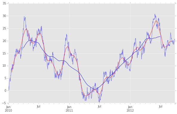
ts = pd.Series(np.random.randn(1000), index=pd.date_range('2010/1/1', periods=1000))
ts = ts.cumsum()
ts.plot(color="b", alpha=0.5, figsize=(10,6))

# 単純移動平均
pd.rolling_mean(ts, 40, center=True).plot(style='-', c='r', alpha=0.8,)
pd.rolling_mean(ts, 180, center=True).plot(style='-', c='blue', alpha=0.9,zorder=100)
# 日付でスライスできる!
ts['2010/12/31':]
out
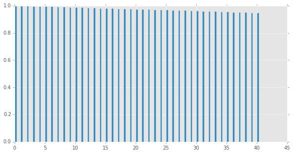
# コレログラムの描画
import statsmodels.tsa.stattools as stt
plt.figure(figsize=(10,5))
acf = stt.acf(np.array(ts), 60) #ACF算出
plt.bar(range(len(acf)), acf, width = 0.3) #表示
plt.show()
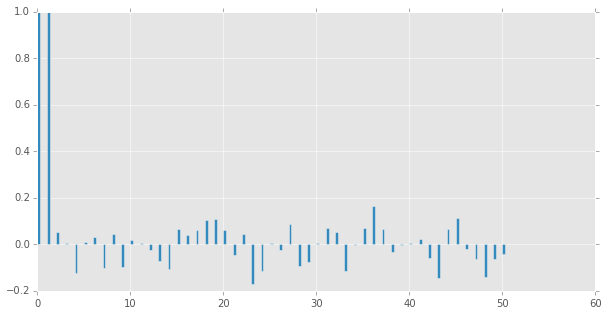
pcf = stt.pacf(np.array(ts), 50)
plt.figure(figsize=(10,5))
plt.bar(range(len(pcf)), pcf, width = 0.3)
plt.show()
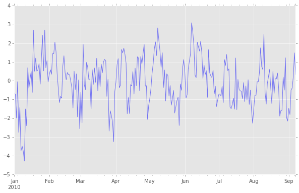
# ARMA(3, 0)過程のサンプル生成
from statsmodels.tsa.arima_process import arma_generate_sample
ar_params = np.array([0.30, 0.50, -0.10])
ma_params = np.array([0.00])
ar_params = np.r_[1, -ar_params]
ma_params = np.r_[1, -ma_params]
nobs = 250
y = arma_generate_sample(ar_params, ma_params, nobs)
ts = pd.Series(y, index=pd.date_range('2010/1/1', periods=nobs))
ts.plot(color="b", alpha=0.5, figsize=(10,6))
plt.figure(figsize=(10,5))
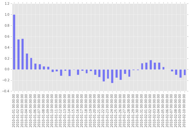
acf = stt.acf(np.array(ts), 60) #ACF算出
ts_acf = pd.Series(acf, index=pd.date_range('2010/1/1', periods=len(acf)))
ts_acf.plot(kind='bar', figsize=(10,5), color="b", alpha=0.5)
plt.show()
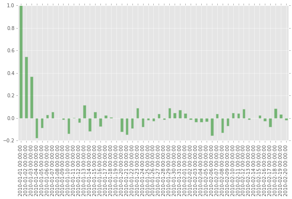
pacf = stt.pacf(np.array(ts), 50)
ts_pacf = pd.Series(pacf, index=pd.date_range('2010/1/1', periods=len(pacf)))
ts_pacf.plot(kind='bar', figsize=(10,5), color="g", alpha=0.5)
plt.show()
import statsmodels.graphics.tsaplots as tsaplots

fig = plt.figure(figsize=(12,5))
ax = fig.add_subplot(111)
tsaplots.plot_acf(ts, ax=ax, color="g")

plt.show()
# ARMA 検定
from statsmodels.tsa import arima_model
arma = arima_model.ARMA(y, order = [3,0]).fit()
print arma.summary()
out
                              ARMA Model Results
==============================================================================
Dep. Variable:                      y   No. Observations:                  250
Model:                     ARMA(3, 0)   Log Likelihood                -357.274
Method:                       css-mle   S.D. of innovations              1.009
Date:                Thu, 13 Aug 2015   AIC                            724.548
Time:                        17:57:45   BIC                            742.155
Sample:                             0   HQIC                           731.634

==============================================================================
                 coef    std err          z      P>|z|      [95.0% Conf. Int.]
------------------------------------------------------------------------------
const          0.0262      0.187      0.140      0.889        -0.341     0.393
ar.L1.y        0.2256      0.063      3.586      0.000         0.102     0.349
ar.L2.y        0.4945      0.057      8.699      0.000         0.383     0.606
ar.L3.y       -0.0569      0.064     -0.895      0.371        -0.181     0.068
                                    Roots
=============================================================================
                 Real           Imaginary           Modulus         Frequency
-----------------------------------------------------------------------------
AR.1            1.2968           +0.0000j            1.2968            0.0000
AR.2           -1.5205           +0.0000j            1.5205            0.5000
AR.3            8.9145           +0.0000j            8.9145            0.0000
-----------------------------------------------------------------------------
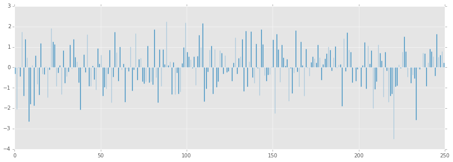
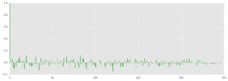
# ARMA残差の確認
resid = arma.resid
plt.figure(figsize=(15,5))
plt.bar(range(len(resid)), resid, width=0.5)
plt.show()
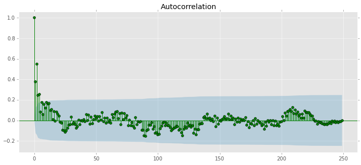
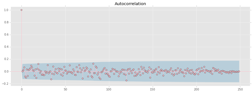
plt.figure(figsize=(15,5))
acf = stt.acf(resid, nlags=len(resid))
plt.bar(range(len(acf)), acf, width=0.5, color="g")
plt.show()
fig = plt.figure(figsize=(15,5))
ax = fig.add_subplot(111)
tsaplots.plot_acf(resid, ax=ax, color="pink")
plt.show()
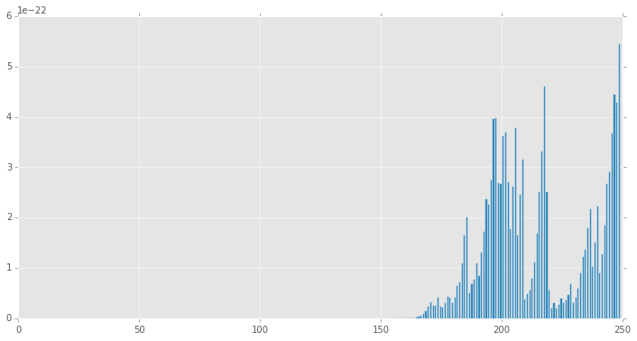
# Ljung-Box Q-statistic for autocorrelation parameters
lbs = stt.q_stat(acf, len(ts))           #statsmodelsはacfを入力とする仕様
plt.figure(figsize=(12,6))
plt.bar(range(len(lbs[1])), lbs[1])
# 欠損値を0で埋める
df_data.fillna(0)
out
out
Spark
import os, sys
from datetime import datetime as dt
print "loading PySpark setting..."
spark_home = os.environ.get('SPARK_HOME', None)
if not spark_home:
    raise ValueError('SPARK_HOME environment variable is not set')
sys.path.insert(0, os.path.join(spark_home, 'python'))
sys.path.insert(0, os.path.join(spark_home, 'python/lib/py4j-0.8.2.1-src.zip'))
execfile(os.path.join(spark_home, 'python/pyspark/shell.py'))
out
loading PySpark setting...
Welcome to
      ____              __
     / __/__  ___ _____/ /__
    _\ \/ _ \/ _ `/ __/  '_/
   /__ / .__/\_,_/_/ /_/\_\   version 1.5.0
      /_/

Using Python version 2.7.10 (default, May 28 2015 17:04:42)
SparkContext available as sc, HiveContext available as sqlContext.
# Cross Validation用にデータを分割
from pyspark.mllib.regression import LabeledPoint

def parsePoint(vec):
    return LabeledPoint(vec[0], vec[1:])

dat = np.column_stack([iris.target[:], iris.data[:,0],iris.data[:,2]])
data = sc.parallelize(dat)   # RDD化
parsedData = data.map(parsePoint)  # 中身のデータをLabeledPointに変換

# 訓練データとテストデータに分割
(trainingData, testData) = parsedData.randomSplit([0.7, 0.3])
out
out
out
out
out
out
out
out
out
out
out
out
out
out
out
out
out
out
out
out
out
out
out
out
out