概要
KerasやTensorflowを使用してニューラルネットワークの重みを計算したものの、それをどうやって実アプリケーション(iPhoneアプリとか、Androidアプリとか、Javascriptとか)に使えば良いのかって、意外と難しい。
単純なニューラルネットワークとなれば、単純で良いのだが、今回LSTMで学習した重みを使用する必要があったので、KerasのLSTMのPredictの内容を解読した。
学習済みの重みはmodel.get_weights()で取ってこれるが、こいつに関する情報がググっても全く出てこない。
結局、コードを書いて、ごちゃごちゃ手当たり次第に試していった結果、model.get_weights()で取ってくる重みは、
1つ目(インデックス0):LSTMの入力層の入力に対する重み、入力ゲートの重み、出力ゲートの重み、忘却ゲートの重み
2つ目(インデックス1):隠れ層の入力に対する重み、入力ゲートの重み、出力ゲートの重み、忘却ゲートの重み
3つ目(インデックス2):入力層、隠れ層に対するバイアス
4つ目(インデックス3):出力層の入力に対する重み(隠れ層の出力に対する重み)
5つ目(インデックス4):出力層に対するバイアス(隠れ層の出力に対するバイアス)
と分かった。
これを解明するために、model.predict()と同様に動きをする(であろう)コードを最後に記述した。
Kerasの公式ページにこういう事が載ってるといいのだが。。。。
get_weigts()の出力
weights = model.get_weights()とすると、以下のような重みが格納されている。
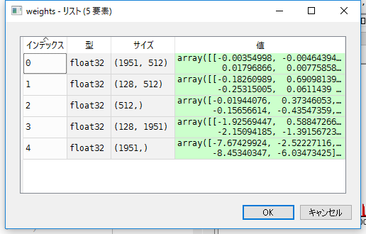
1951という数字は入力層のノード数なので、問題ない。
インデックス3の128も、隠れ層のノード数を128に設定しているので、隠れ層の出力に対する重みだと分かる。
問題は512で、こいつが一番混乱した。
パッと思いついたのは、「入力に対する重み、入力ゲートの重み、出力ゲートの重み、忘却ゲートの重み」の4種類が格納されてるという予想。
しかし、Kerasの公式ページを見ると、LSTMは(長短期記憶ユニット - Hochreiter 1997.)を使用しているという記載がある。
あれ、1997といえば、忘却ゲートに重みがなかったんじゃなかったっけ。。。?
忘却ゲートができたのは、1999だったような。。。。
ここにもそう書いてあるよね・・・・?
http://kivantium.hateblo.jp/entry/2016/01/31/222050
それで混乱しつつも、ベタ打ちでコードを書けば、こいつらが解明されると思って、model.predictと同じ挙動をする今回のコードを書くことに。
model.predict()を解明するコード
前提として、今回解読に使用したLSTMのmodelは以下。LSTMを用いて、文章を生成するサンプルコード。
from __future__ import print_function
from keras.models import Sequential
from keras.layers import Dense, Activation
from keras.layers import LSTM
from keras.optimizers import RMSprop
from keras.utils.data_utils import get_file
import numpy as np
import random
import sys
from keras.models import model_from_json
import copy
import matplotlib.pyplot as plt
import math

#path = get_file('nietzsche.txt', origin='https://s3.amazonaws.com/text-datasets/nietzsche.txt')
text = open('hokkaido_x.txt', 'r', encoding='utf8').read().lower()
print('corpus length:', len(text))

chars = sorted(list(set(text)))
print('total chars:', len(chars))
char_indices = dict((c, i) for i, c in enumerate(chars))
indices_char = dict((i, c) for i, c in enumerate(chars))

# cut the text in semi-redundant sequences of maxlen characters
#maxlen = 40
maxlen = 3
step = 2
sentences = []
next_chars = []
for i in range(0, len(text) - maxlen, step):
    sentences.append(text[i: i + maxlen])
    next_chars.append(text[i + maxlen])
print('nb sequences:', len(sentences))

print('Vectorization...')
X = np.zeros((len(sentences), maxlen, len(chars)), dtype=np.bool)
y = np.zeros((len(sentences), len(chars)), dtype=np.bool)
for i, sentence in enumerate(sentences):
    for t, char in enumerate(sentence):
        X[i, t, char_indices[char]] = 1
    y[i, char_indices[next_chars[i]]] = 1


# build the model: a single LSTM
print('Build model...')
model = Sequential()
model.add(LSTM(128, input_shape=(maxlen, len(chars)),activation='sigmoid',inner_activation='sigmoid'))
model.add(Dense(len(chars)))
model.add(Activation('softmax'))

optimizer = RMSprop(lr=0.01)
model.compile(loss='categorical_crossentropy', optimizer=optimizer)


def sample(preds, temperature=1.0):
    # helper function to sample an index from a probability array
    preds = np.asarray(preds).astype('float64')
    preds = np.log(preds) / temperature
    exp_preds = np.exp(preds)
    preds = exp_preds / np.sum(exp_preds)
    probas = np.random.multinomial(1, preds, 1)
    return np.argmax(probas)


model.fit(X, y, batch_size=64, epochs=1)

diversity = 0.5
print()

generated = ''
sentence = "ゴジラ"
#    sentence = text[start_index: start_index + maxlen]
generated += sentence
  #        print('----- Generating with seed: "' + sentence + '"')
  #  sys.stdout.write(generated)

  #        for i in range(400):
x = np.zeros((1, maxlen, len(chars)))
for t, char in enumerate(sentence):
    x[0, t, char_indices[char]] = 1.

preds = model.predict(x, verbose=0)[0]

plt.plot(preds,'r-')
plt.show()
これに対して、model.predictと同じ値を出力するのが以下のコード。for文を書くのも疲れてしまったので、c1,c2,c3などと記載しているが、これらの数は上記modelのmaxlenに対応している。maxlenを増やしたければ、for文書いてループ構造を組めばよい。
コードとかは以下のサイトを参考にさせてもらった。
http://blog.yusugomori.com/post/154208605320/javascript%E3%81%AB%E3%82%88%E3%82%8Bdeep-learning%E3%81%AE%E5%AE%9F%E8%A3%85long-short-term
print(preds)

weights = model.get_weights()


obj=weights

w1=obj[0]
w2=obj[1]
w3=obj[2]
w4=obj[3]
w5=obj[4]

hl = 128

def sigmoid(x):
    return 1.0 / (1.0 + np.exp(-x))

def tanh(x):
    return (np.exp(x)-np.exp(-x))/(np.exp(x)+np.exp(-x))

def activate(x):
    x[0:hl] = sigmoid(x[0:hl]) #i
    x[hl:hl*2] = sigmoid(x[hl:hl*2]) #a
    x[hl*2:hl*3] = sigmoid(x[hl*2:hl*3]) #f
    x[hl*3:hl*4] = sigmoid(x[hl*3:hl*4]) #o
    return x

def cactivate(c):
    return sigmoid(c)

x1 = np.array(x[0,0,:])
x2 = np.array(x[0,1,:])
x3 = np.array(x[0,2,:])

h1 = np.zeros(hl)
c1 = np.zeros(hl)

o1 = x1.dot(w1)+h1.dot(w2)+w3
o1 = activate(o1)

c1 = o1[0:hl]*o1[hl:hl*2] + o1[hl*2:hl*3]*c1
#c1 = o1[0:128]*o1[128:256] + c1

h2 = o1[hl*3:hl*4]*cactivate(c1)

#2個目
o2 =  x2.dot(w1)+h2.dot(w2)+w3
o2 = activate(o2)

c2 = o2[0:hl]*o2[hl:hl*2] + o2[hl*2:hl*3]*c1
#c2 = o2[0:128]*o2[128:256] + c1

h3 = o2[hl*3:hl*4]*cactivate(c2)

#3個目
o3 = x3.dot(w1)+h3.dot(w2)+w3
o3 = activate(o3)

c3 = o3[0:hl]*o3[hl:hl*2] + o3[hl*2:hl*3]*c2
#c3 = o3[0:128]*o3[128:256] + c2

h4 = o3[hl*3:hl*4]*cactivate(c3)

y = h4.dot(w4)+w5

y = np.exp(y)/np.sum(np.exp(y))

plt.plot(y,'b-')
plt.show()
結果、predsとyが同様の値を出力するのがわかる。
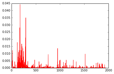
predsのプロット結果
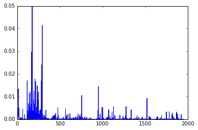
yのプロット結果
ちなみに上記コードは活性化関数、内部セル関数ともにsigmoidとしているが、tanhではなぜか上手くいかなかった。解決したらアップデートしたい。