pythonを使って、フライトシミュレータなど常微分方程式形式になっている物理モデルのシミュレーション(数値解析・数値計算)をする方法。
やっていることはScipy.integrateの中にあるodeintを使う。FortranのOdepackのlsodeを使っているらしいので、計算は早い。
例
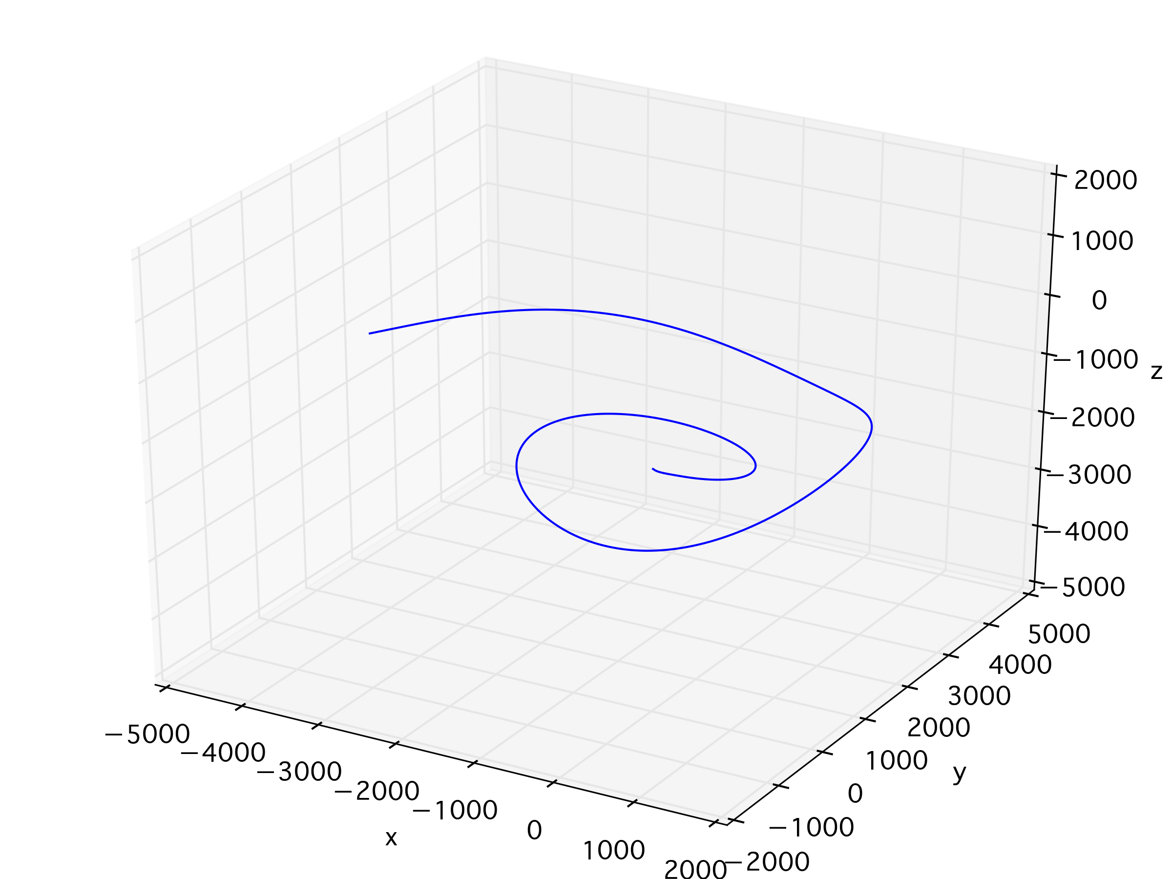
例としてOctave(Matlab互換)のコードとして公開されている飛行機のフライトシミュレーションをpythonに移植してみる。計算の中身についてはリンク先が詳しい。
Butterfly_Effect( ) 6DOF Flight Simulation
時間経過によって動くもののシミュレーションをするのに、forを使ってしまうとオイラー法など簡単な数値計算法であってもpythonではかなり遅いのでなるべくscipyなどのライブラリを使うべき。
matlabとpythonの違い
matlabからの移植をするときは行列(ndarray)の*演算子がmatlab:内積、numpy:要素積と違うので注意。また、pythonでは小数点を明示しないと整数除算になってしまうので注意が必要。
コード - odeint
# -*- coding: utf-8 -*-
import numpy as np
from scipy.integrate import odeint
from scipy.linalg import block_diag
import matplotlib.pyplot as plt
from mpl_toolkits.mplot3d import Axes3D

plt.close('all')

# import time
# start = time.time()

def Rotation_X(Psi):
	R_x = np.array([[np.cos(Psi), np.sin(Psi), 0],
					[-np.sin(Psi), np.cos(Psi), 0],
					[0, 0, 1]])
	return R_x

def Rotation_Y(Theta):
	R_y = np.array([[np.cos(Theta), 0, -np.sin(Theta)],
					[0, 1, 0],
					[np.sin(Theta), 0, np.cos(Theta)]])
	return R_y

def Rotation_Z(Phi):
	R_z = np.array([[1, 0, 0],
					[0, np.cos(Phi), np.sin(Phi)],
					[0, -np.sin(Phi), np.cos(Phi)]])
	return R_z

# 運動方程式
def dynamical_system(x, t, A, U0):
	# x = [u,alpha,q,theta,beta,p,r,phi,psi,x,y,z]
	dx = A.dot(x)
	u = x[0]+U0 # 速度
	UVW = np.array([u, u*x[4], u*x[1]]) # 速度ベクトル[U,V,W]
	Rotation = Rotation_X(-x[8]).dot(Rotation_Y(-x[3])).dot(Rotation_Z(-x[7]))
	dX = Rotation.dot(UVW)
	dx[9]  = dX[0]
	dx[10] = dX[1]
	dx[11] = dX[2]
	return dx

# 有次元安定微係数
Xu = -0.01;   Zu = -0.1;   Mu = 0.001
Xa = 30.0;    Za = -200.0; Ma = -4.0
Xq = 0.3;     Zq = -5.0;   Mq = -1.0
Yb = -45.0;   Lb_= -2.0;   Nb_= 1.0
Yp = 0.5;     Lp_= -1.0;   Np_= -0.1
Yr = 3.0;     Lr_= 0.2;    Nr_=-0.2

# その他のパラメタ
W0 = 0.0;     U0 = 100.0;  theta0 = 0.05
g  = 9.8 # 重力加速度

# 縦のシステム
A_lat = np.array([[Xu, Xa, -W0, -g*np.cos(theta0)],
    			  [Zu/U0, Za/U0, (U0+Zq)/U0, -g*np.sin(theta0)/U0],
    			  [Mu, Ma, Mq, 0],
    			  [0, 0, 1, 0]])

# 横・方向のシステム
A_lon = np.array([[Yb, (W0+Yp), -(U0-Yr), g*np.cos(theta0), 0],
        		  [Lb_, Lp_, Lr_, 0, 0],
        		  [Nb_, Np_, Nr_, 0, 0],
        		  [0, 1, np.tan(theta0), 0, 0],
        		  [0, 0, 1/np.cos(theta0), 0, 0]])

# 対角ブロックとしてシステムを結合する
A = block_diag(A_lat, A_lon)

# さらに飛行軌道分のスペースを確保しておく
A = block_diag(A, np.zeros([3,3]))

# 計算条件の設定
endurance	= 200	# 飛行時間[sec]
step		= 10	# 1.0[sec]あたりの時間ステップ数
t = np.linspace(0,endurance,endurance*step)

# 初期値 x0 = [u,alpha,q,theta, beta,p,r,phi,psi]
# 常微分方程式に入れる変数は1次元にする必要がある。
x0_lat		= np.array([10, 0.1, 0.4, 0.2])		# 縦の初期値
x0_lon		= np.array([0.0, 0.6, 0.4, 0.2, 0.2])	# 横・方向の初期値
x0_pos		= np.array([0, 0, -1000]) # 飛行機の初期位置
x0 = np.hstack((x0_lat, x0_lon, x0_pos))

x = odeint(dynamical_system, x0, t, args=(A,U0,))
print u"run successfully."

# 可視化
plt.ion()
fig = plt.figure()
ax = Axes3D(fig)

ax.plot(x[:,9], x[:,10], x[:,11])
ax.set_xlabel(u"x");ax.set_ylabel(u"y");ax.set_zlabel(u"z")
ax.set_xlim([-5000,2000])
ax.set_ylim([-2000,5000])
ax.set_zlim([-5000,2000])
plt.show()
コード - ode
scipy.integrateの中にはodeintだけではなく、オブジェクト指向で作られているodeという常微分方程式の数値計算の汎用的なインターフェイスもある。
odeintと違って、計算方法が指定できるので、計算の中身を決めたい場合はこちらが良い。また、計算を途中で終わらせることも出来そう。
ただし、whileで計算を回しているのでstep数にもよるが計算スピードがかなり遅い。手元の環境では10倍程度遅かった。また、微分方程式の関数の引数の順番が(時間、変数)とodeintと逆になってたり、タプルの引数にしないといけなかったりと、細々違うので注意必要。
# -*- coding: utf-8 -*-
import numpy as np
from scipy.integrate import odeint
from scipy.integrate import ode
from scipy.linalg import block_diag
import matplotlib.pyplot as plt
from mpl_toolkits.mplot3d import Axes3D

plt.close('all')

def Rotation_X(Psi):
	R_x = np.array([[np.cos(Psi), np.sin(Psi), 0],
					[-np.sin(Psi), np.cos(Psi), 0],
					[0, 0, 1]])
	return R_x

def Rotation_Y(Theta):
	R_y = np.array([[np.cos(Theta), 0, -np.sin(Theta)],
					[0, 1, 0],
					[np.sin(Theta), 0, np.cos(Theta)]])
	return R_y

def Rotation_Z(Phi):
	R_z = np.array([[1, 0, 0],
					[0, np.cos(Phi), np.sin(Phi)],
					[0, -np.sin(Phi), np.cos(Phi)]])
	return R_z

# 運動方程式
# odeintの場合と違って(time, x, args*)なこと、及びargsがタプルなことに注意
def dynamical_system(t, x, (A, U0)):
	# x = [u,alpha,q,theta,beta,p,r,phi,psi,x,y,z]
	dx = A.dot(x)
	u = x[0]+U0 # 速度
	UVW = np.array([u, u*x[4], u*x[1]]) # 速度ベクトル[U,V,W]
	Rotation = Rotation_X(-x[8]).dot(Rotation_Y(-x[3])).dot(Rotation_Z(-x[7]))
	dX = Rotation.dot(UVW)
	dx[9]  = dX[0]
	dx[10] = dX[1]
	dx[11] = dX[2]
	return dx

# 有次元安定微係数
Xu = -0.01;   Zu = -0.1;   Mu = 0.001
Xa = 30.0;    Za = -200.0; Ma = -4.0
Xq = 0.3;     Zq = -5.0;   Mq = -1.0
Yb = -45.0;   Lb_= -2.0;   Nb_= 1.0
Yp = 0.5;     Lp_= -1.0;   Np_= -0.1
Yr = 3.0;     Lr_= 0.2;    Nr_=-0.2

# その他のパラメタ
W0 = 0.0;     U0 = 100.0;  theta0 = 0.05
g  = 9.8 # 重力加速度

# 縦のシステム
A_lat = np.array([[Xu, Xa, -W0, -g*np.cos(theta0)],
    			  [Zu/U0, Za/U0, (U0+Zq)/U0, -g*np.sin(theta0)/U0],
    			  [Mu, Ma, Mq, 0],
    			  [0, 0, 1, 0]])

# 横・方向のシステム
A_lon = np.array([[Yb, (W0+Yp), -(U0-Yr), g*np.cos(theta0), 0],
        		  [Lb_, Lp_, Lr_, 0, 0],
        		  [Nb_, Np_, Nr_, 0, 0],
        		  [0, 1, np.tan(theta0), 0, 0],
        		  [0, 0, 1/np.cos(theta0), 0, 0]])

# 対角ブロックとしてシステムを結合する
A = block_diag(A_lat, A_lon)

# さらに飛行軌道分のスペースを確保しておく
A = block_diag(A, np.zeros([3,3]))

# 計算条件の設定
endurance	= 200	# 飛行時間[sec]
step		= 10	# 1.0[sec]あたりの時間ステップ数
dt 			= 1.0 / step 	# 時間ステップの幅[sec]
t0 			= 0.0	# 開始時間[sec]
t = np.linspace(0,endurance,endurance*step)

# 初期値 x0 = [u,alpha,q,theta, beta,p,r,phi,psi,x,y,z]
# 常微分方程式に入れる変数は1次元にする必要がある。
x0_lat		= np.array([10, 0.1, 0.4, 0.2])		# 縦の初期値
x0_lon		= np.array([0.0, 0.6, 0.4, 0.2, 0.2])	# 横・方向の初期値
x0_pos		= np.array([0, 0, -1000]) # 飛行機の初期位置
x0 = np.hstack((x0_lat, x0_lon, x0_pos))

# ODEの設定
solver = ode(dynamical_system).set_integrator('vode', method='bdf')
solver.set_initial_value(x0, t0)
solver.set_f_params((A, U0))
dt = 1.0 / step
x = np.zeros([int(endurance/dt)+1, 12])
t = np.zeros([int(endurance/dt)+1])

index = 0
while solver.successful() and solver.t < endurance:
	solver.integrate(solver.t+dt)
	x[index] = solver.y
	t[index] = solver.t
	index += 1

print u"run successfully."

# 可視化
plt.ion()
fig = plt.figure()
ax = Axes3D(fig)

ax.plot(x[:,9], x[:,10], x[:,11])
ax.set_xlim([-5000,2000])
ax.set_ylim([-2000,5000])
ax.set_zlim([-5000,2000])
plt.show()