はじめに
画像認識などで広く使われている畳み込みニューラルネットワーク(Convolutional Neural Networks, CNN)ですが、
最近は自然言語処理の分野でも使われています [Kim, EMNLP2014]。
今回は、ChainerでCNNを使った簡単なネットワークを構築し、文書分類のタスクに適用してみました。
データの置き場
- 今回実装したソースコード
- 実験に使用したデータ
事前準備
- Chainer, scikit-learn, gensimのインストール
- word2vecの学習済みモデル( GoogleNews-vectors-negative300.bin.gz)のダウンロード.
環境
- Python 2.7系
- Chainer 1.6.2.1
文書ベクトルの作成
今回は、入力文書をword2vecを用いてベクトル化し、ベクトル化された文書に対して畳み込みを行います。
文書のベクトル化はuitl.pyに定義しているdef load_data(fname)で行っています。
イメージとしては、入力された何らかの単語列(文書) $x_1$,$x_2$,$x_3$, .... , $x_n$ の各単語$x_i$を
固定次元$N$のベクトルに変換し、それらを並べた2次元の文書ベクトルを作成します。
[例]
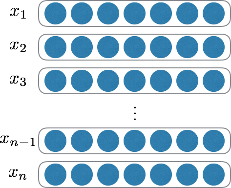
また、文書ごとに文長が異なるため、入力文書の中で最大の文長$maxlen$に合わせるためにpaddingを行います。
つまり、生成される2次元の文書ベクトルの次元は、$N * maxlen$となります。
ちなみに、今回使用したGoogleが公開しているword2vecのモデルでは、各単語ベクトルの次元は300です。
def load_data(fname):
    # 学習済みのword2vecモデルを読み込み
    model =  word2vec.Word2Vec.load_word2vec_format('GoogleNews-vectors-negative300.bin', binary=True)

    target = [] #ラベル
    source = [] #文書ベクトル

    #文書リストを作成
    document_list = []
    for l in open(fname, 'r').readlines():
        sample = l.strip().split(' ',  1)
        label = sample[0]
        target.append(label) #ラベル
        document_list.append(sample[1].split()) #文書ごとの単語リスト

    max_len = 0
    rev_document_list = [] #未知語処理後のdocument list
    for doc in document_list:
        rev_doc = []
        for word in doc:
            try:
                word_vec = np.array(model[word]) #未知語の場合, KeyErrorが起きる
                rev_doc.append(word)
            except KeyError:
                rev_doc.append('<unk>') #未知語
        rev_document_list.append(rev_doc)
        #文書の最大長を求める(padding用)
        if len(rev_doc) > max_len:
            max_len = len(rev_doc)

    #文書長をpaddingにより合わせる
    rev_document_list = padding(rev_document_list, max_len)

    width = 0 #各単語の次元数
    #文書の特徴ベクトル化
    for doc in rev_document_list:
        doc_vec = []
        for word in doc:
            try:
                vec = model[word.decode('utf-8')]
            except KeyError:
                vec = model.seeded_vector(word)
            doc_vec.extend(vec)
            width = len(vec)
        source.append(doc_vec)

    dataset = {}
    dataset['target'] = np.array(target)
    dataset['source'] = np.array(source)

    return dataset, max_len, width
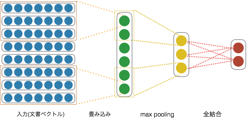
モデルの定義
今回は、畳み込み層->プーリング層->全結合層という構成のモデルを定義しました。
途中でドロップアウトもかませています。
class SimpleCNN(Chain):

    def __init__(self, input_channel, output_channel, filter_height, filter_width, mid_units, n_units, n_label):
        super(SimpleCNN, self).__init__(
            conv1 = L.Convolution2D(input_channel, output_channel, (filter_height, filter_width)),
            l1    = L.Linear(mid_units, n_units),
            l2    = L.Linear(n_units,  n_label),
        )

    #Classifier によって呼ばれる
    def __call__(self, x):
        h1 = F.max_pooling_2d(F.relu(self.conv1(x)), 3)
        h2 = F.dropout(F.relu(self.l1(h1)))
        y = self.l2(h2)
        return y
学習
学習では、1エポック毎に訓練データとテストデータそれぞれで正解率、ロスを計算して表示させています。
フィードフォワードニューラルネットワークを使って文書分類した時とほぼ同じコードになっています。
畳み込み時の、フィルタサイズは3×300(各単語ベクトルの次元数)にしています。
# Prepare dataset
dataset, height, width = util.load_data(args.data)
print 'height:', height
print 'width:', width

dataset['source'] = dataset['source'].astype(np.float32) #特徴量
dataset['target'] = dataset['target'].astype(np.int32) #ラベル

x_train, x_test, y_train, y_test = train_test_split(dataset['source'], dataset['target'], test_size=0.15)
N_test = y_test.size         # test data size
N = len(x_train)             # train data size
in_units = x_train.shape[1]  # 入力層のユニット数 (語彙数)

# (nsample, channel, height, width) の4次元テンソルに変換
input_channel = 1
x_train = x_train.reshape(len(x_train), input_channel, height, width)
x_test  = x_test.reshape(len(x_test), input_channel, height, width)

# 隠れ層のユニット数
n_units = args.nunits
n_label = 2
filter_height = 3
output_channel = 50

# モデルの定義
model = L.Classifier( SimpleCNN(input_channel, output_channel, filter_height, width, 950, n_units, n_label))

# GPUを使うかどうか
if args.gpu > 0:
    cuda.check_cuda_available()
    cuda.get_device(args.gpu).use()
    model.to_gpu()
    xp = np if args.gpu <= 0 else cuda.cupy #args.gpu <= 0: use cpu, otherwise: use gpu

batchsize = args.batchsize
n_epoch = args.epoch

# Setup optimizer
optimizer = optimizers.AdaGrad()
optimizer.setup(model)

# Learning loop
for epoch in six.moves.range(1, n_epoch + 1):

    print 'epoch', epoch, '/', n_epoch

    # training)
    perm = np.random.permutation(N) #ランダムな整数列リストを取得
    sum_train_loss     = 0.0
    sum_train_accuracy = 0.0
    for i in six.moves.range(0, N, batchsize):

        #perm を使い x_train, y_trainからデータセットを選択 (毎回対象となるデータは異なる)
        x = chainer.Variable(xp.asarray(x_train[perm[i:i + batchsize]])) #source
        t = chainer.Variable(xp.asarray(y_train[perm[i:i + batchsize]])) #target

        optimizer.update(model, x, t)

        sum_train_loss      += float(model.loss.data) * len(t.data)   # 平均誤差計算用
        sum_train_accuracy  += float(model.accuracy.data ) * len(t.data)   # 平均正解率計算用

    print('train mean loss={}, accuracy={}'.format(sum_train_loss / N, sum_train_accuracy / N)) #平均誤差

    # evaluation
    sum_test_loss     = 0.0
    sum_test_accuracy = 0.0
    for i in six.moves.range(0, N_test, batchsize):

        # all test data
        x = chainer.Variable(xp.asarray(x_test[i:i + batchsize]))
        t = chainer.Variable(xp.asarray(y_test[i:i + batchsize]))

        loss = model(x, t)

        sum_test_loss     += float(loss.data) * len(t.data)
        sum_test_accuracy += float(model.accuracy.data)  * len(t.data)

    print(' test mean loss={}, accuracy={}'.format(
        sum_test_loss / N_test, sum_test_accuracy / N_test)) #平均誤差

    if epoch > 10:
        optimizer.lr *= 0.97
        print 'learning rate: ', optimizer.lr

    sys.stdout.flush()
実験結果
最終的な正解率は、accuracy=0.775624996424となりました。
フィードフォワードニューラルネットワークで分類した時は、accuracy=0.716875001788だったので、かなり正解率が良くなりました。
(フィードフォワードニューラルネットのときは、word2vecは使わず、one hotな単語ベクトルを使って文書ベクトルを作っていたので、実験の条件は異なります。)
height: 59
width: 300
epoch 1 / 100
train mean loss=0.68654858897, accuracy=0.584814038988
 test mean loss=0.673290403187, accuracy=0.674374999106
epoch 2 / 100
train mean loss=0.653146019086, accuracy=0.678733030628
 test mean loss=0.626838338375, accuracy=0.695624998212
epoch 3 / 100
train mean loss=0.604344114544, accuracy=0.717580840894
 test mean loss=0.582373640686, accuracy=0.713124997914

...

epoch 98 / 100
train mean loss=0.399981137426, accuracy=0.826288489978
 test mean loss=0.460177404433, accuracy=0.775625003874
learning rate:  6.85350312961e-05
epoch 99 / 100
train mean loss=0.400466494895, accuracy=0.822536144887
 test mean loss=0.464013618231, accuracy=0.773749999702
learning rate:  6.64789803572e-05
epoch 100 / 100
train mean loss=0.399539747416, accuracy=0.824081227461
 test mean loss=0.466326575726, accuracy=0.775624996424
learning rate:  6.44846109465e-05
save the model
save the optimizer
おわりに
畳み込みニューラルネットワークを使って、文書分類(ポジネガ分類)をしてみました。
シンプルなモデルでしたが、それなりの精度はでるようです。
次は、 Yoon Kimのモデルもchainerで実装したので、
記事を投稿しようと思います。