Rでニュートンラフソン法を実装

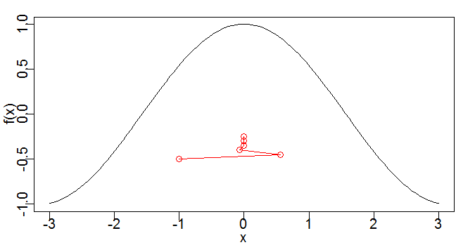
これなら分かる最適化数学 3.2 に記載の通り、ニュートンラフソン法（ニュートン法）を用いて、関数に最大値・最小値を取らせる変数の値を求めます。

1変数の場合

frame()
par(mfcol=c(1, 1))
par(mar=c(2, 2, 1, 0.1))
par(mgp=c(1, 0.2, 0))
xrange <- c(-3, 3)
yrange <- c(-1, 1)
f <- function(x) { cos(x) }
dx <- function(x) { -sin(x) }
dxdx <- function(x) { -cos(x) }
newton <- function(x0, f, df, d2f) {

    x <- x0
    eps <- 1e-6
    i <- 1
    # 解の移動量が十分小さくなるまで繰り返す。
    repeat {
        oldx <- x
        x <- x - df(x) / d2f(x)
        lines(c(oldx, x), c(i - 1, i) * 0.05 - 0.5, type="o", col=2)
        cat("i=", i, "x=" , x, "f(x)=", f(x), "df(x)=", df(x), "\n")
        if (abs(x - oldx) < eps) {
            break
        }
        i <- i + 1
    }
    x
}

curve(f, xlim=range(xrange), ylim=range(yrange))
newton(-1, f, dx, dxdx)

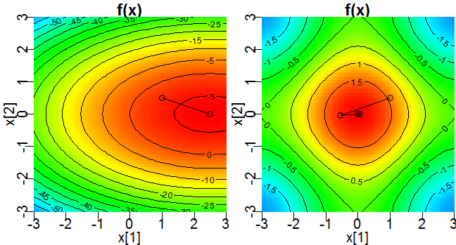
多変数の場合

frame()
par(mfcol=c(1, 2))
par(mar=c(2, 2, 1, 0.1))
par(mgp=c(1, 0.2, 0))

newton <- function(x0, f, df, dxdx, dxdy, dydx, dydy) {

    x <- x0
    eps <- 1e-12
    i <- 1
    repeat {
        oldx <- x
        # 勾配∇fを求める。
        gradientf <- c(dx(x), dy(x))
        # ヘッセ行列Hを求める。
        H <- matrix(c(dxdx(x), dxdy(x), dydx(x), dydy(x)), 2, byrow=T)
        # HΔx=-∇fを解き、Δx=-H^-1 ∇fを求める。
        deltax <- solve(H, -gradientf)
        x <- x + deltax
        xy <- cbind(oldx, x)
        lines(xy[1, ], xy[2, ], type="o", col=1)
        cat("i=", i, "x=" , x, "f(x)=", f(x), "df(x)=", df(x), "\n")
        # ||Δx||^2 が十分小さくなるまで繰り返す。
        if (sum(deltax * deltax) < eps) {
            break
        }
        i <- i + 1
    }
    x
}

draw <- function() {
    xgrid <- seq(-3, 3, 0.1)
    ygrid <- seq(-3, 3, 0.1)
    zgrid <- outer(xgrid, ygrid, Vectorize(function(x, y){ f(c(x, y)) }))
    image(xgrid, ygrid, zgrid, xlim=range(xgrid), ylim=range(ygrid), xlab="x[1]", ylab="x[2]", main="f(x)", col=rainbow(450)[256:1])
    contour(xgrid, ygrid, zgrid, xlim=range(xgrid), ylim=range(ygrid), add=T)
    newton(c(1, 0.5), f, dx, dxdx, dxdy, dydx, dydy)
}

f <- function(x){ -x[1] ^ 2 - 4 * x[2] ^ 2 + 5 * x[1] }
dx <- function(x){ -2 * x[1] + 5 }
dy <- function(x){ - 8 * x[2] }
dxdx <- function(x){ -2 }
dxdy <- function(x){ 0 }
dydx <- function(x){ 0 }
dydy <- function(x){ -8 }
draw()

f <- function(x){ cos(x[1]) + cos(x[2]) }
dx <- function(x){ -sin(x[1]) }
dy <- function(x){ -sin(x[2]) }
dxdx <- function(x){ -cos(x[1]) }
dxdy <- function(x){ 0 }
dydx <- function(x){ 0 }
dydy <- function(x){ -cos(x[2]) }
draw()

# f <- function(x){ x[1] ^ 3 + x[2] ^ 3 - 9 * x[1] * x[2] + 27 }
# dx <- function(x){ 3 * x[1] ^ 2 - 9 * x[2] }
# dy <- function(x){ 3 * x[2] ^ 2 - 9 * x[1] }
# dxdx <- function(x){ 6 * x[1] }
# dxdy <- function(x){ -9 }
# dydx <- function(x){ -9 }
# dydy <- function(x){ 6 * x[2] }
# draw()