はじめに

Chainer 1.16.0 のリリースでNStepLSTMが実装されました。
NStepLSTMはその名のとおりLSTMの多層化が容易に実現できるモデルとなっています。
内部的にはcuDNNで最適化されたRNNが使われており、従来のLSTMに比べて高速に動作します。
さらにNStepLSTMではミニバッチのデータの長さをそろえる必要がなくなり、各サンプルをリストに入れたものをそのまま入力できるようになりました。
これまでのように-1でpaddingしてignore_label=-1とwhereを駆使したり、データの長さ順にソートしたリストを転置して入力したりという手順が不要になりました。

そこで今回はこのNStepLSTMを使って系列ラベリングの学習をしてみました。

従来のLSTMとのインタフェースの違い

NStepLSTMはこれまでのLSTMと入出力が異なるので、今まで実装したモデルを単にNStepLSTMで置き換えるということができません。

NStepLSTMの__init__()と__call__()の入出力は次のようになっています。

NStepLSTM.__init__(n_layers, in_size, out_size, dropout, use_cudnn=True)
"""
n_layers (int): Number of layers.
in_size (int): Dimensionality of input vectors.
out_size (int): Dimensionality of hidden states and output vectors.
dropout (float): Dropout ratio.
use_cudnn (bool): Use cuDNN.
"""

...

NStepLSTM.__call__(hx, cx, xs, train=True)
"""
hx (~chainer.Variable): Initial hidden states.
cx (~chainer.Variable): Initial cell states.
xs (list of ~chianer.Variable): List of input sequences.
        Each element ``xs[i]`` is a :class:`chainer.Variable` holding a sequence.
"""
    ...

    return hy, cy, ys

対して従来のLSTMは以下のようでした。

LSTM.__init__(in_size, out_size, **kwargs)
"""
in_size (int) – Dimension of input vectors. If None, parameter initialization will be deferred until the first forward data pass at which time the size will be determined.
out_size (int) – Dimensionality of output vectors.
lateral_init – A callable that takes numpy.ndarray or cupy.ndarray and edits its value.
        It is used for initialization of the lateral connections.
        Maybe be None to use default initialization.
upward_init – A callable that takes numpy.ndarray or cupy.ndarray and edits its value.
        It is used for initialization of the upward connections.
        Maybe be None to use default initialization.
bias_init – A callable that takes numpy.ndarray or cupy.ndarray and edits its value.
        It is used for initialization of the biases of cell input, input gate and output gate, and gates of the upward connection.
        Maybe a scalar, in that case, the bias is initialized by this value.
        Maybe be None to use default initialization.
forget_bias_init – A callable that takes numpy.ndarray or cupy.ndarray and edits its value.
        It is used for initialization of the biases of the forget gate of the upward connection.
        Maybe a scalar, in that case, the bias is initialized by this value.
        Maybe be None to use default initialization.
"""

...

LSTM.__call__(x)
"""
x (~chainer.Variable): A new batch from the input sequence.
"""
    ...

    return y

したがって、NStepLSTMは以下の点でLSTMと取扱いが異なります。

__init()__でlayer数とdropout ratioを指定する
__call()__で初期のhidden statesと初期のcell statesを渡さないといけない
__call()__の入力はchainer.Variableではなくchainer.Variableのリスト
__call()__の返り値は系列のforward計算をし終えたあとのhidden states, cell statesとoutput (chainer.Variable)のリスト

__call()__の呼び出しに初期のhidden statesとcell statesを与えること、入出力がリストになっていることが大きく違います。

NStepLSTMを取扱いやすくする

NStepLSTMの初期化と呼び出しをなるべくLSTMに近づけるようにサブクラスを実装します。

#!/usr/bin/env python
# -*- coding: utf-8 -*-

from chainer import Variable
import chainer.links as L
import numpy as np


class LSTM(L.NStepLSTM):

    def __init__(self, in_size, out_size, dropout=0.5, use_cudnn=True):
        n_layers = 1
        super(LSTM, self).__init__(n_layers, in_size, out_size, dropout, use_cudnn)
        self.state_size = out_size
        self.reset_state()

    def to_cpu(self):
        super(LSTM, self).to_cpu()
        if self.cx is not None:
            self.cx.to_cpu()
        if self.hx is not None:
            self.hx.to_cpu()

    def to_gpu(self, device=None):
        super(LSTM, self).to_gpu(device)
        if self.cx is not None:
            self.cx.to_gpu(device)
        if self.hx is not None:
            self.hx.to_gpu(device)

    def set_state(self, cx, hx):
        assert isinstance(cx, Variable)
        assert isinstance(hx, Variable)
        cx_ = cx
        hx_ = hx
        if self.xp == np:
            cx_.to_cpu()
            hx_.to_cpu()
        else:
            cx_.to_gpu()
            hx_.to_gpu()
        self.cx = cx_
        self.hx = hx_

    def reset_state(self):
        self.cx = self.hx = None

    def __call__(self, xs, train=True):
        batch = len(xs)
        if self.hx is None:
            xp = self.xp
            self.hx = Variable(
                xp.zeros((self.n_layers, batch, self.state_size), dtype=xs[0].dtype),
                volatile='auto')
        if self.cx is None:
            xp = self.xp
            self.cx = Variable(
                xp.zeros((self.n_layers, batch, self.state_size), dtype=xs[0].dtype),
                volatile='auto')

        hy, cy, ys = super(LSTM, self).__call__(self.hx, self.cx, xs, train)
        self.hx, self.cx = hy, cy
        return ys

上記のクラスでは__init()__はこれまでどおりin_size, out_sizeのみ指定（dropoutのデフォルト値は0.5, LSTMの多層化はせずにn_layers=1に固定）というふうにしました。
__call()__はcx, hxを自動で初期化し、入出力はchainer.Variableのリストのみにしました。

NStepLSTMでBi-directional LSTMを実装

NStepLSTMを使ってBi-directional LSTMを実装します。
forward-LSTMに渡すchainer.Variableのリストの各サンプルを反対向きにしてbackward-LSTMの入力用のリストを作ります。
forward-LSTMとbackward-LSTMでoutputを計算したあと、それぞれの出力のリストの各サンプルの向きをそろえてconcatenateしてひとつのベクトルにします。
下のクラスでは系列ラベリング用にout_sizeがラベル数になるように線形の演算を加えています。

class BLSTMBase(Chain):

    def __init__(self, embeddings, n_labels, dropout=0.5, train=True):
        vocab_size, embed_size = embeddings.shape
        feature_size = embed_size
        super(BLSTMBase, self).__init__(
            embed=L.EmbedID(
                in_size=vocab_size,
                out_size=embed_size,
                initialW=embeddings,
            ),
            f_lstm=LSTM(feature_size, feature_size, dropout),
            b_lstm=LSTM(feature_size, feature_size, dropout),
            linear=L.Linear(feature_size * 2, n_labels),
        )
        self._dropout = dropout
        self._n_labels = n_labels
        self.train = train

    def reset_state(self):
        self.f_lstm.reset_state()
        self.b_lstm.reset_state()

    def __call__(self, xs):
        self.reset_state()
        xs_f = []
        xs_b = []
        for x in xs:
            _x = self.embed(self.xp.array(x))
            xs_f.append(_x)
            xs_b.append(_x[::-1])
        hs_f = self.f_lstm(xs_f, self.train)
        hs_b = self.b_lstm(xs_b, self.train)
        ys = [self.linear(F.dropout(F.concat([h_f, h_b[::-1]]), ratio=self._dropout, train=self.train)) for h_f, h_b in zip(hs_f, hs_b)]
        return ys

Bi-directional LSTMを使って系列ラベリングの学習をする

上で実装したモデルを実際に使って系列ラベリングのタスクに適用してみます。
Bi-directional LSTMがよく使われている系列ラベリングの問題として、中国語のWord Segmentationを選択しました。
中国語は英語のようにスペースで単語が区切られていないため、テキストを処理する前に語の境界を同定する必要があります。

例)

冬天 (winter)，能 (can) 穿 (wear) 多少 (amount) 穿 (wear) 多少 (amount)；
夏天 (summer)，能 (can) 穿 (wear) 多 (more) 少 (little) 穿 (wear) 多 (more) 少 (little)。

[Chen+, 2015]

上記の例は"多少"と区切るか"多"と"少"に区切るかで意味が異なる例です。
文の構造としてはほぼ同じなので前後の単語との文脈で区切りを判定します。

系列ラベリングの問題として中国語の単語分割を学習するために、文字列に対してB(Begin, 2文字以上の単語の先頭), M(Middle, 2文字以上の単語の真ん中), E(End, 2文字以上の単語の終端), S(Single, 1文字の単語)の4つのラベルを振っていきます。
このラベルが付与されたテキストデータを使って、単語列の文脈情報から各文字に割り当てられるラベルを学習していきます。

実験

対象のデータセット

PKU (Peking University corpus, 中国語Word Segmentationのベンチマークのための標準的なデータセット）

環境

Python 3.5.2
Chainer 1.18.0
Ubuntu 14.04.5 LTS + GPU

モデル & 実験設定

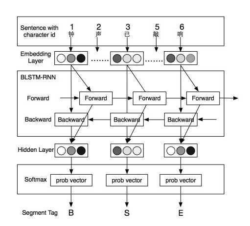
[Yao+, 2016] ※上図モデルと酷似 ¹

Bi-directional LSTM
epoch: 10
dropout ratio: 0.5
AdaGrad - learning rate: 0.2
weight decay: 10^-4
ミニバッチのサイズ: 20
Word Embeddingsのpretrain: Chinese Wikipedia corpus, 100 dim

実験結果

本モデルの学習過程と結果

学習の過程を以下にそのまま記載します。

hiroki-t:/private/work/blstm-cws$ python app/train.py --save -e 10 --gpu 0
2016-12-03 09:34:06.27 JST      13a653  [info]  LOG Start with ACCESSID=[13a653] UNIQUEID=[UNIQID] ACCESSTIME=[2016-12-03 09:34:06.026907 JST]
2016-12-03 09:34:06.27 JST      13a653  [info]  *** [START] ***
2016-12-03 09:34:06.27 JST      13a653  [info]  initialize preprocessor with /private/work/blstm-cws/app/../data/zhwiki-embeddings-100.txt
2016-12-03 09:34:06.526 JST     13a653  [info]  load train dataset from /private/work/blstm-cws/app/../data/icwb2-data/training/pku_training.utf8
2016-12-03 09:34:14.134 JST     13a653  [info]  load test dataset from /private/work/blstm-cws/app/../data/icwb2-data/gold/pku_test_gold.utf8
2016-12-03 09:34:14.589 JST     13a653  [trace]
2016-12-03 09:34:14.589 JST     13a653  [trace] initialize ...
2016-12-03 09:34:14.589 JST     13a653  [trace] --------------------------------
2016-12-03 09:34:14.589 JST     13a653  [info]  # Minibatch-size: 20
2016-12-03 09:34:14.589 JST     13a653  [info]  # epoch: 10
2016-12-03 09:34:14.589 JST     13a653  [info]  # gpu: 0
2016-12-03 09:34:14.589 JST     13a653  [info]  # hyper-parameters: {'adagrad_lr': 0.2, 'dropout_ratio': 0.2, 'weight_decay': 0.0001}
2016-12-03 09:34:14.590 JST     13a653  [trace] --------------------------------
2016-12-03 09:34:14.590 JST     13a653  [trace]
100% (19054 of 19054) |#######################################| Elapsed Time: 0:07:50 Time: 0:07:50
2016-12-03 09:42:05.642 JST     13a653  [info]  [training] epoch 1 - #samples: 19054, loss: 9.640346, accuracy: 0.834476
100% (1944 of 1944) |#########################################| Elapsed Time: 0:00:29 Time: 0:00:29
2016-12-03 09:42:34.865 JST     13a653  [info]  [evaluation] epoch 1 - #samples: 1944, loss: 6.919845, accuracy: 0.890557
2016-12-03 09:42:34.866 JST     13a653  [trace] -
100% (19054 of 19054) |#######################################| Elapsed Time: 0:07:40 Time: 0:07:40
2016-12-03 09:50:15.258 JST     13a653  [info]  [training] epoch 2 - #samples: 19054, loss: 5.526157, accuracy: 0.903373
100% (1944 of 1944) |#########################################| Elapsed Time: 0:00:24 Time: 0:00:24
2016-12-03 09:50:39.400 JST     13a653  [info]  [evaluation] epoch 2 - #samples: 1944, loss: 6.233129, accuracy: 0.900318
2016-12-03 09:50:39.401 JST     13a653  [trace] -
100% (19054 of 19054) |#######################################| Elapsed Time: 0:08:41 Time: 0:08:41
2016-12-03 09:59:21.301 JST     13a653  [info]  [training] epoch 3 - #samples: 19054, loss: 4.217260, accuracy: 0.921377
100% (1944 of 1944) |#########################################| Elapsed Time: 0:00:24 Time: 0:00:24
2016-12-03 09:59:45.587 JST     13a653  [info]  [evaluation] epoch 3 - #samples: 1944, loss: 5.650668, accuracy: 0.913843
2016-12-03 09:59:45.587 JST     13a653  [trace] -
100% (19054 of 19054) |#######################################| Elapsed Time: 0:07:25 Time: 0:07:25
2016-12-03 10:07:11.451 JST     13a653  [info]  [training] epoch 4 - #samples: 19054, loss: 3.488712, accuracy: 0.931668
100% (1944 of 1944) |#########################################| Elapsed Time: 0:00:26 Time: 0:00:26
2016-12-03 10:07:37.889 JST     13a653  [info]  [evaluation] epoch 4 - #samples: 1944, loss: 5.342249, accuracy: 0.917103
2016-12-03 10:07:37.890 JST     13a653  [trace] -
100% (19054 of 19054) |#######################################| Elapsed Time: 0:07:26 Time: 0:07:26
2016-12-03 10:15:03.919 JST     13a653  [info]  [training] epoch 5 - #samples: 19054, loss: 2.995683, accuracy: 0.938305
100% (1944 of 1944) |#########################################| Elapsed Time: 0:00:15 Time: 0:00:15
2016-12-03 10:15:19.749 JST     13a653  [info]  [evaluation] epoch 5 - #samples: 1944, loss: 5.320374, accuracy: 0.921863
2016-12-03 10:15:19.750 JST     13a653  [trace] -
100% (19054 of 19054) |########################################| Elapsed Time: 0:07:29 Time: 0:07:29
2016-12-03 10:22:49.393 JST     13a653  [info]  [training] epoch 6 - #samples: 19054, loss: 2.680496, accuracy: 0.943861
100% (1944 of 1944) |##########################################| Elapsed Time: 0:00:27 Time: 0:00:27
2016-12-03 10:23:16.985 JST     13a653  [info]  [evaluation] epoch 6 - #samples: 1944, loss: 5.326864, accuracy: 0.924161
2016-12-03 10:23:16.986 JST     13a653  [trace] -
100% (19054 of 19054) |########################################| Elapsed Time: 0:07:28 Time: 0:07:28
2016-12-03 10:30:45.772 JST     13a653  [info]  [training] epoch 7 - #samples: 19054, loss: 2.425466, accuracy: 0.947673
100% (1944 of 1944) |##########################################| Elapsed Time: 0:00:22 Time: 0:00:22
2016-12-03 10:31:08.448 JST     13a653  [info]  [evaluation] epoch 7 - #samples: 1944, loss: 5.270019, accuracy: 0.925341
2016-12-03 10:31:08.449 JST     13a653  [trace] -
100% (19054 of 19054) |########################################| Elapsed Time: 0:08:39 Time: 0:08:39
2016-12-03 10:39:47.461 JST     13a653  [info]  [training] epoch 8 - #samples: 19054, loss: 2.233068, accuracy: 0.950928
100% (1944 of 1944) |##########################################| Elapsed Time: 0:00:26 Time: 0:00:26
2016-12-03 10:40:14.2 JST       13a653  [info]  [evaluation] epoch 8 - #samples: 1944, loss: 5.792994, accuracy: 0.924707
2016-12-03 10:40:14.2 JST       13a653  [trace] -
100% (19054 of 19054) |########################################| Elapsed Time: 0:07:10 Time: 0:07:10
2016-12-03 10:47:24.806 JST     13a653  [info]  [training] epoch 9 - #samples: 19054, loss: 2.066807, accuracy: 0.953524
100% (1944 of 1944) |##########################################| Elapsed Time: 0:00:26 Time: 0:00:26
2016-12-03 10:47:51.745 JST     13a653  [info]  [evaluation] epoch 9 - #samples: 1944, loss: 5.864374, accuracy: 0.925294
2016-12-03 10:47:51.746 JST     13a653  [trace] -
100% (19054 of 19054) |########################################| Elapsed Time: 0:08:43 Time: 0:08:43
2016-12-03 10:56:34.758 JST     13a653  [info]  [training] epoch 10 - #samples: 19054, loss: 1.946193, accuracy: 0.955782
100% (1944 of 1944) |##########################################| Elapsed Time: 0:00:22 Time: 0:00:22
2016-12-03 10:56:57.641 JST     13a653  [info]  [evaluation] epoch 10 - #samples: 1944, loss: 5.284819, accuracy: 0.930201
2016-12-03 10:56:57.642 JST     13a653  [trace] -
2016-12-03 10:56:57.642 JST     13a653  [info]  saving the model to /private/work/blstm-cws/app/../output/cws.model ...
2016-12-03 10:56:58.520 JST     13a653  [info]  *** [DONE] ***
2016-12-03 10:56:58.521 JST     13a653  [info]  LOG End with ACCESSID=[13a653] UNIQUEID=[UNIQID] ACCESSTIME=[2016-12-03 09:34:06.026907 JST] PROCESSTIME=[4972.494370000]

Precision, Recall, F値ではなくAccuracyの値ですが、10epoch目で93.0となっています。
処理時間は10epochで80分強という結果となりました。

先行研究の結果と比較

[Yao+, 2016] ²

All the models are trained on NVIDIA GTX Geforce 970, it took about 16 to 17 hours to train a model on GPU while more than 4 days to train on CPU, in contrast.

[Yao+, 2016]

Embeddingsの初期化など先行研究と少し異なる点はありますが、1層のBLSTMの精度と処理時間としてはまずまずの結果ではないでしょうか。

Decoding

hiroki-t:/private/work/blstm-cws$ python app/parse.py
2016-12-03 11:01:13.343 JST     549e15  [info]  LOG Start with ACCESSID=[549e15] UNIQUEID=[UNIQID] ACCESSTIME=[2016-12-03 11:01:13.343412 JST]
2016-12-03 11:01:13.343 JST     549e15  [info]  *** [START] ***
2016-12-03 11:01:13.344 JST     549e15  [info]  initialize preprocessor with /private/work/blstm-cws/app/../data/zhwiki-embeddings-100.txt
2016-12-03 11:01:13.834 JST     549e15  [trace]
2016-12-03 11:01:13.834 JST     549e15  [trace] initialize ...
2016-12-03 11:01:13.834 JST     549e15  [trace]
2016-12-03 11:01:13.914 JST     549e15  [info]  loading a model from /private/work/blstm-cws/app/../output/cws.model ...
Input a Chinese sentence! (use 'q' to exit)
中国人民进入了向现代化建设第三步战略目标迈进的新征程。
B E B E B E S S B M E B E B E S B E B E B E S S B E S
中国 人民 进入 了 向 现代化 建设 第三 步 战略 目标 迈进 的 新 征程 。
-
q
2016-12-03 11:02:08.961 JST     549e15  [info]  *** [DONE] ***
2016-12-03 11:02:08.962 JST     549e15  [info]  LOG End with ACCESSID=[549e15] UNIQUEID=[UNIQID] ACCESSTIME=[2016-12-03 11:01:13.343412 JST] PROCESSTIME=[55.618552000]

# ^注 [gold] 中国  人民  进入  了  向  现代化  建设  第三  步  战略  目标  迈进  的  新  征程  。

学習結果をもとにdecodingをすると分割されていない文字列から正しいラベル系列と単語分割の結果が返ってきました。

おわりに

ChainerのNStepLSTMを使ってBi-directional LSTMで系列ラベリングの学習をしました。
可変長なミニバッチ+cuDNN対応でこれまでよりも入力データの処理が楽になり、演算も高速になりました。
今回実装したモデルは中国語の単語分割に限らず系列学習に汎用的に使えるので、品詞タグ付けなど別のタスクにも応用してみると面白いかもしれません。

ソースコードはGitHubで公開しています。
https://github.com/chantera/blstm-cws

リポジトリには上記で紹介したBLSTMに加えて、BLSTM+CRFの実装やNLPの研究で私が実際にChainerと組み合わせて使っているコードを置いていますので参考になれば幸いです。

参考

可変長データのミニバッチをchainerのwhereでやる - studylog/北の雲 http://studylog.hateblo.jp/entry/2016/02/04/020547
ChainerのcuDNN-RNN(NStepLSTM)のとっかかり - studylog/北の雲 http://studylog.hateblo.jp/entry/2016/10/03/095406
ChainerのNStepLSTMでニコニコ動画のコメント予測。 - Monthly Hacker's Blog http://www.monthly-hack.com/entry/2016/10/24/200000
chainer-NStepLSTM/ptb_nslstm.py at master · monthly-hack/chainer-NStepLSTM https://github.com/monthly-hack/chainer-NStepLSTM/blob/master/ptb_nslstm.py
LSTMの可変長系列入力について - Google グループ https://groups.google.com/forum/#!topic/chainer-jp/og0dBbgSLVw
Optimizing Recurrent Neural Networks in cuDNN 5 | Parallel Forall https://devblogs.nvidia.com/parallelforall/optimizing-recurrent-neural-networks-cudnn-5/
Chen, X., Qiu, X., Zhu, C., Liu, P. and Huang, X., 2015. Long short-term memory neural networks for chinese word segmentation. In Proceedings of the Conference on Empirical Methods in Natural Language Processing (pp. 1385-1394). http://aclweb.org/anthology/D15-1141.pdf
Huang, Z., Xu, W., Yu, K., 2015. Bidirectional LSTM-CRF models for sequence tagging. arXiv preprint arXiv:1508.01991. https://arxiv.org/abs/1508.01991
Yao, Y., Huang, Z., 2016. Bi-directional LSTM Recurrent Neural Network for Chinese Word Segmentation. arXiv preprint arXiv:1602.04874. https://arxiv.org/abs/1602.04874

written by chantera at NAIST cllab

[Yao+, 2016] ではBLSTMの出力のベクトルv ∈ R^2dをW ∈ R^d*2dの行列でd次元に戻している。 ↩
[Yao+, 2016] ではWord Embeddingsのdimensionを200次元に設定しており、pretrainをせずにtrainingセットの文字から辞書を作っている ↩

可変長ミニバッチを使ったChainerの系列学習の実装