An Introduction to Statistical Learningの第三章に相関係数を使う一例があったので,まとめます.
広告の投資(TV, Radio, Newspaper)と売上(Sales)関連性を示すデータ・セットを使っています.
CSVファイルをimportして,最初の5行を表示します.
%matplotlib inline
import pandas as pd
import statsmodels.formula.api as smf
import seaborn as sns
import matplotlib.pyplot as plt

advertising = pd.read_csv("http://www-bcf.usc.edu/~gareth/ISL/Advertising.csv", usecols=[1,2,3,4])
advertising.head()
このデータセットは200行あって,カラムは4つです.
advertising.shape

# 結果
# (200, 4)
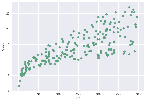
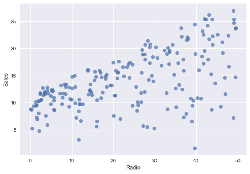
まずTV,Radio,NewspaperそれぞれSalesとの関連性をグラフで見てみます. それぞれのグラフのx軸は違うことに注意必要です.
TV ~ Sales
plt.scatter(advertising.TV , advertising.Sales,  alpha=0.7)
plt.xlabel("TV")
plt.ylabel("Sales")
plt.show()
Radio ~ Sales
plt.scatter(advertising.Radio , advertising.Sales,  alpha=0.7)
plt.xlabel("Radio")
plt.ylabel("Sales")
plt.show()
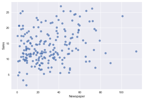
Newspaper ~ Sales
plt.scatter(advertising.Newspaper , advertising.Sales,  alpha=0.7)
plt.xlabel("Newspaper")
plt.ylabel("Sales")
plt.show()
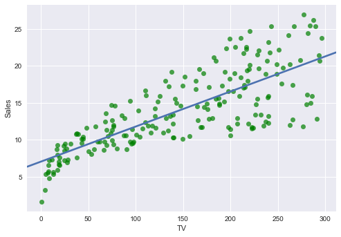
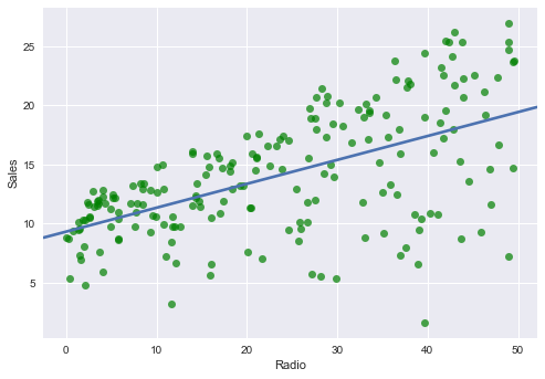
上の図を参考に仮にTV, Radio, NewspaperそれぞれSalesと線形回帰の関係もっているとします.グラフをプロットしてみます.
TV ~ Sales
sns.regplot(advertising.TV, advertising.Sales, ci=None, scatter_kws={'color':'g', 'alpha':0.7})
plt.xlabel("TV")
plt.ylabel("Sales")
plt.show()
Radio ~ Sales
sns.regplot(advertising.Radio, advertising.Sales, ci=None, scatter_kws={'color':'g', 'alpha':0.7})
plt.xlabel("Radio")
plt.ylabel("Sales")
plt.show()
Newspaper ~ Sales
sns.regplot(advertising.Newspaper, advertising.Sales, ci=None, scatter_kws={'color':'g', 'alpha':0.7})
plt.xlabel("Newspaper")
plt.ylabel("Sales")
plt.show()
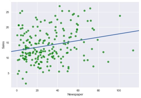
なんとなく TV〜Sales 回帰直線の傾きが大きいで, Newspaper〜Sales 回帰直線の傾きが小さいです.
TV ~ Sales回帰直線の傾き(coefficient)とy切片(intercept)をscikit learnのLinearRegressionで求めてみる.
from sklearn.linear_model import LinearRegression

reg = LinearRegression()

X = advertising.TV.values.reshape(-1,1)
y = advertising.Sales

reg.fit(X,y)

print("intercept: ", reg.intercept_)
print("coefficient: ", reg.coef_)
結果:
intercept:  7.03259354913
coefficient:  [ 0.04753664]
Radio ~ Sales回帰直線の傾き(coefficient)とy切片(intercept)をscikit learnのLinearRegressionで求めてみる.
from sklearn.linear_model import LinearRegression

reg = LinearRegression()

X = advertising.Radio.values.reshape(-1,1)
y = advertising.Sales

reg.fit(X,y)

print("intercept: ", reg.intercept_)
print("coefficient: ", reg.coef_)
結果:
intercept:  9.31163809516
coefficient:  [ 0.20249578]
Newspaper ~ Sales回帰直線の傾き(coefficient)とy切片(intercept)をscikit learnのLinearRegressionで求めてみる.
from sklearn.linear_model import LinearRegression

reg = LinearRegression()

X = advertising.Newspaper.values.reshape(-1,1)
y = advertising.Sales

reg.fit(X,y)

print("intercept: ", reg.intercept_)
print("coefficient: ", reg.coef_)
結果:
intercept:  12.3514070693
coefficient:  [ 0.0546931]
Newspaper ~ Sales回帰直線の傾き(coefficient)に注目すると, 0.0546931になっています.
つまりNewspaperへの広告投資はSalesへ貢献無視できない. でもホントそうなのかは検証してみたいです.
さっきTV,Radio,Newspaperそれぞれ単回帰をscikit learn検証しました.今回多重回帰で検証してみます.
from sklearn.linear_model import LinearRegression

reg = LinearRegression()

X = advertising[['TV', 'Radio', 'Newspaper']].as_matrix()
y = advertising.Sales

reg.fit(X,y)

print("intercept: ", reg.intercept_)
print("coefficient: ", reg.coef_)
結果:
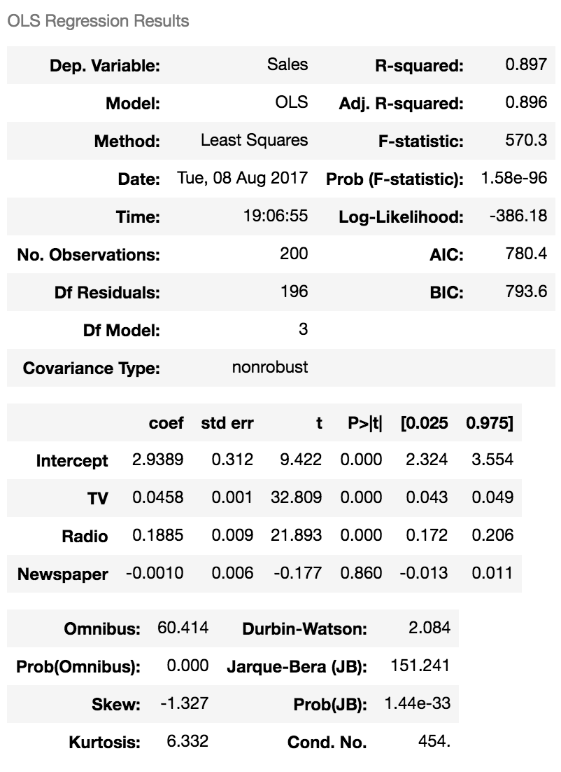
intercept:  2.93888936946
coefficient:  [ 0.04576465  0.18853002 -0.00103749]
TV,Radioのcoefficientの部分さっき単回帰で検証した結果あんまり変わっていないです.
ここで興味深いのは Newspaperの coefficientは -0.00103749になりました.つまりNewspaperへの広告投資はSalseへの影響はないと? 実際はそうです.
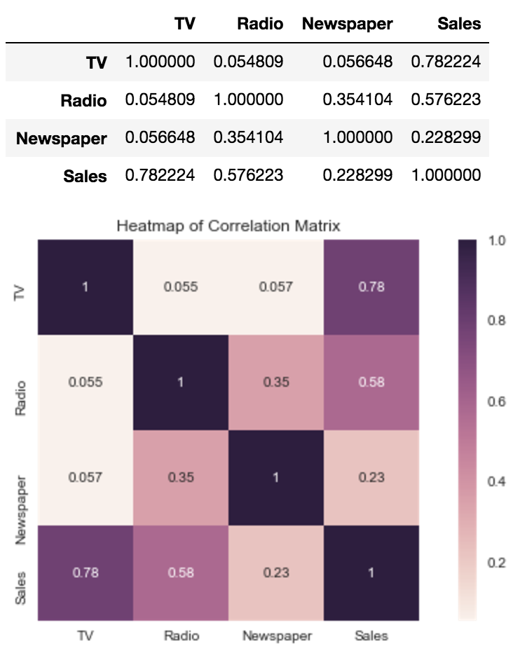
4つの変数の相関関係を見てみます. NewspaperとSalesの相関係数は一番小さいです.さらに NewspaperとRadioの相関係数0.354104は大きめです.Radioへの広告投資は多くなると,Newspaperへの広告投資も増えます. RadioとSalesの相関係数大きいです. つまりNewspaper〜Sales単回帰で求めたcoefficient 0.0546931実はRadioの恩恵を受けて,関連性あるように見えただけです.
単回帰は他の要素の影響を無視しているので,出てきた結論は一部間違いがあることがわかりました.
corr = advertising.corr()

plt.figure(figsize=(10,5))

sns.heatmap(corr,
            xticklabels=corr.columns.values,
            yticklabels=corr.columns.values,
            vmax=1,
            square=True,
            annot=True
           )
sns.plt.title('Heatmap of Correlation Matrix')
corr
さっきのinterceptとcoefficient見づらいなら,したの方法で求めることもできます. 下の2個目の表のNewspaperのp値0.860は非常に大きい値で, Newspaper〜Salesの間に関連性がないことの裏付けになります.
est = smf.ols('Sales ~ TV + Radio + Newspaper', advertising).fit()
est.summary()