動作環境
GeForce GTX 1070 (8GB)
ASRock Z170M Pro4S [Intel Z170chipset]
Ubuntu 14.04 LTS desktop amd64
TensorFlow v0.11
cuDNN v5.1 for Linux
CUDA v8.0
Python 2.7.6
IPython 5.1.0 -- An enhanced Interactive Python.
gcc (Ubuntu 4.8.4-2ubuntu1~14.04.3) 4.8.4
GNU bash, version 4.3.8(1)-release (x86_64-pc-linux-gnu)
v0.1: http://qiita.com/7of9/items/09262a2ab01d037d169b
概要
This article is related to ADDA (light scattering simulator based on the discrete dipole approximation).
ADDAの計算で重要となるのが、X,Y,Z方向の電場の値。ランダムな初期値を用いると計算が遅く、最終の解に近い初期値を用いると計算が早くなることは経験済。
supercomputerで計算した最終解を元にDeep learningで学習を行い、その結果を通常のPCで用いる。そうすることで、通常のPC上での計算を高速化し、Communityとしての計算資源の効率利用を目論んでいる。
X,Y,Z方向の電場の値をTensorFlowで学習させようとしている。
学習コード: v0.2
v0.1: X方向の実部のみを学習。
v0.2 (今回): X方向の実部と虚部を学習。
実部と虚部の同時学習はv0.1に至るまでのテストコードで失敗をしていた。今回、再確認のため実施してみた。
データの準備
v0.1を参照: http://qiita.com/7of9/items/09262a2ab01d037d169b
diff
diff --git a/learnExr_170422.py b/learnExr_170422.py
index 98f8c24..cd64426 100644
--- a/learnExr_170422.py
+++ b/learnExr_170422.py
@@ -11,6 +11,7 @@ import numpy as np

 '''
 v0.3 Mar. 03, 2017
+  - learn [Exr] and [Exi]
   - add [Eyr, Eri, Ezr, Ezi] for decode_csv()
 v0.2 Apr. 29, 2017
   - save to [model_variables_170429.npy]
@@ -48,7 +49,7 @@ def_rec = [[0.], [0.], [0.], [0.], [0.], [0.], [0.], [0.], [0.]]
 wrk = tf.decode_csv(value, record_defaults=def_rec)
 xpos, ypos, zpos, Exr, Exi, Eyr, Eyi, Ezr, Ezi = wrk
 inputs = tf.pack([xpos, ypos, zpos])
-output = tf.pack([Exr])
+output = tf.pack([Exr, Exi])

 batch_size = 4  # [4]
 # Ref: cifar10_input.py
@@ -62,13 +63,13 @@ inputs_batch, output_batch = tf.train.shuffle_batch(
     min_after_dequeue=batch_size)

 input_ph = tf.placeholder("float", [None, 3])
-output_ph = tf.placeholder("float", [None, 1])
+output_ph = tf.placeholder("float", [None, 2])

 ## network
 hiddens = slim.stack(input_ph, slim.fully_connected, [100, 100, 100],
                      activation_fn=tf.nn.sigmoid, scope="hidden")
 prediction = slim.fully_connected(
-    hiddens, 1, activation_fn=None, scope="output")
+    hiddens, 2, activation_fn=None, scope="output")
 loss = tf.contrib.losses.mean_squared_error(prediction, output_ph)

 train_op = slim.learning.create_train_op(loss, tf.train.AdamOptimizer(0.001))
全コード
learnExr_170422.py
# !/usr/bin/env python
# -*- coding: utf-8 -*-

from __future__ import absolute_import
from __future__ import division
from __future__ import print_function
import sys
import tensorflow as tf
import tensorflow.contrib.slim as slim
import numpy as np

'''
v0.3 Mar. 03, 2017
  - learn [Exr] and [Exi]
  - add [Eyr, Eri, Ezr, Ezi] for decode_csv()
v0.2 Apr. 29, 2017
  - save to [model_variables_170429.npy]
  - learn [Exr] only, instead of [Exr, Exi]
v0.1 Apr. 23, 2017
  - change [NUM_EXAMPLES_PER_EPOCH_FOR_TRAIN] from [100] to [9328]
  - change input layer's node from [2] to [3]
  - [input.csv] has 9 columns
=== branched from [learn_xxyyfunc_170321.py] to [learnExr_170422.py] ===
v0.5 Apr. 01, 2017
  - change network from [7,7,7] to [100, 100, 100]
v0.4 Mar. 31, 2017
  - calculate [capacity] from [min_queue_examples] and [batch_size]
v0.3 Mar. 24, 2017
  - change [capacity] from 100 to 40
v0.2 Mar. 24, 2017
  - change [capacity] from 40 to 100
  - output [model_variables] after training
v0.1 Mar. 22, 2017
  - learn mapping of R^2 input to R^2 output
     + using data prepared by [prep_data_170321.py]
  - branched from sine curve learning at
    http://qiita.com/7of9/items/ce58e66b040a0795b2ae
'''

# codingrule:PEP8


filename_queue = tf.train.string_input_producer(["input.csv"])

# prase CSV
reader = tf.TextLineReader()
key, value = reader.read(filename_queue)
def_rec = [[0.], [0.], [0.], [0.], [0.], [0.], [0.], [0.], [0.]]
wrk = tf.decode_csv(value, record_defaults=def_rec)
xpos, ypos, zpos, Exr, Exi, Eyr, Eyi, Ezr, Ezi = wrk
inputs = tf.pack([xpos, ypos, zpos])
output = tf.pack([Exr, Exi])

batch_size = 4  # [4]
# Ref: cifar10_input.py
min_fraction_of_examples_in_queue = 0.2  # 0.4
NUM_EXAMPLES_PER_EPOCH_FOR_TRAIN = 9328
min_queue_examples = int(NUM_EXAMPLES_PER_EPOCH_FOR_TRAIN *
                         min_fraction_of_examples_in_queue)
#
inputs_batch, output_batch = tf.train.shuffle_batch(
    [inputs, output], batch_size, capacity=min_queue_examples + 3 * batch_size,
    min_after_dequeue=batch_size)

input_ph = tf.placeholder("float", [None, 3])
output_ph = tf.placeholder("float", [None, 2])

## network
hiddens = slim.stack(input_ph, slim.fully_connected, [100, 100, 100],
                     activation_fn=tf.nn.sigmoid, scope="hidden")
prediction = slim.fully_connected(
    hiddens, 2, activation_fn=None, scope="output")
loss = tf.contrib.losses.mean_squared_error(prediction, output_ph)

train_op = slim.learning.create_train_op(loss, tf.train.AdamOptimizer(0.001))

init_op = tf.initialize_all_variables()

with tf.Session() as sess:
    coord = tf.train.Coordinator()
    threads = tf.train.start_queue_runners(sess=sess, coord=coord)

    try:
        sess.run(init_op)
        for i in range(90000):  # 30000
            inpbt, outbt = sess.run([inputs_batch, output_batch])
            _, t_loss = sess.run([train_op, loss],
                                 feed_dict={input_ph: inpbt, output_ph: outbt})

            if (i+1) % 100 == 0:
                print("%d,%f" % (i+1, t_loss))
                sys.stdout.flush()

    finally:
        coord.request_stop()

    # output the model
    model_variables = slim.get_model_variables()
    res = sess.run(model_variables)
    np.save('model_variables_170429.npy', res)

    coord.join(threads)
実行
$python learnExr_170422.py > res.learn_170503
lossの経過
Jupyter code.
check_result_170423.ipynb
%matplotlib inline

# learning [Exr] from ADDA
# Mar. 03, 2017

import numpy as np
import matplotlib.pyplot as plt

# data1 = np.loadtxt('res.learn_170423', delimiter=',')
# data1 = np.loadtxt('res.learn_170429', delimiter=',')
data1 = np.loadtxt('res.learn_170503', delimiter=',')

input1 = data1[:,0]
output1 = data1[:,1]

fig = plt.figure()
ax1 = fig.add_subplot(2,1,1)

ax1.plot(input1, output1)

ax1.set_xlabel('step')
ax1.set_ylabel('loss')
ax1.set_ylim([0,0.05])
ax1.grid(True)

fig.show()
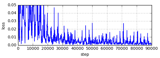
順調にlossが減少している。
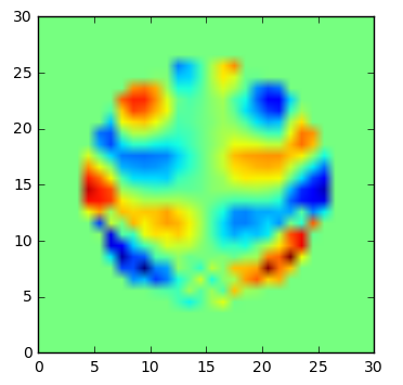
学習結果
Exの実部 (学習対象)
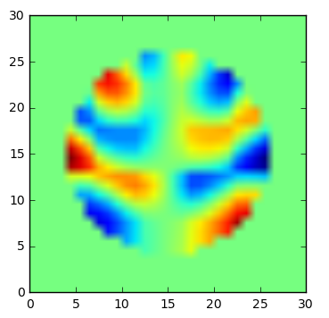
Exの実部 (学習結果)
Exの虚部 (学習対象)
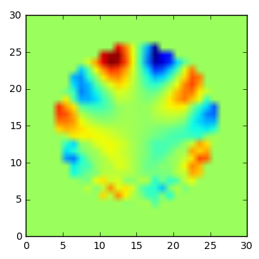
Exの虚部 (学習結果)
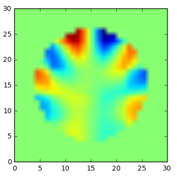
学習できている。
今週はここらでつまずく予定だったが、STYX HELIXが良かったのだろうか。