Environment
GeForce GTX 1070 (8GB)
ASRock Z170M Pro4S [Intel Z170chipset]
Ubuntu 14.04 LTS desktop amd64
TensorFlow v0.11
cuDNN v5.1 for Linux
CUDA v8.0
Python 2.7.6
IPython 5.1.0 -- An enhanced Interactive Python.
gcc (Ubuntu 4.8.4-2ubuntu1~14.04.3) 4.8.4
GNU bash, version 4.3.8(1)-release (x86_64-pc-linux-gnu)
This article is related to ADDA (light scattering simulator based on the discrete dipole approximation).
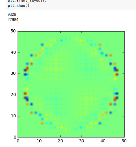
In this article, pvec[] (polarization of dipoles) is displayed in 2D.
Reference: https://groups.google.com/forum/#!topic/adda-discuss/f3_Cm3HFtkA
Required
- UtilReadCoordinate.py
- UtilReadCheckPoint.py
- Coordinate file: coord.0
- produced with modified
iterative.c
- produced with modified
coord.0 was produced with the following:
$ ./adda -grid 25 -chp_type normal -chpoint 1s > log
v0.3
code
Jupyter code
displayPvec_170410.py
from mpl_toolkits.mplot3d import Axes3D
import matplotlib.pyplot as plt
import matplotlib.cm as cm
import numpy as np
import sys

from UtilReadCoordinate import read_coordinate_file
from UtilReadCheckPoint import read_chpoint_file

'''
v0.3 Apr. 15, 2017
   - display pvec[::3] in 2D
v0.2 Apr. 14, 2017
   - use [sys.float_info.epsilon] for float comparison
v0.1 Apr. 10, 2017
   - read checkpoint file
   - read coordinate file
'''

res = read_coordinate_file('coord.0')
local_nvoid_Ndip, coord = res
res = read_chpoint_file('chp.0', 'aux.0')
itrgrp, auxgrp, vecgrp = res

print(local_nvoid_Ndip)
print(len(vecgrp.pvec))

xs, ys, zs = coord[::3], coord[1::3], coord[2::3]
pvc1, pvc2, pvc3 = vecgrp.pvec[::3], vecgrp.pvec[1::3], vecgrp.pvec[2::3]

plt_y1 = np.array([])
PICK_UP_ZZ_VALUE = -0.20943951023931953

SIZE_MAP_X, SIZE_MAP_Y = 50, 50
MIN_X, MIN_Y = -6, -6  # -6: based on coordinate values
RANGE_X = 6 - MIN_X  # 6: based on coordinate values
RANGE_Y = 6 - MIN_Y  # 6: based on coordinate values
rmap = [[0.0 for yi in range(SIZE_MAP_Y)] for xi in range(SIZE_MAP_X)]

for idx, xyz in enumerate(zip(xs, ys, zs)):
    xx, yy, zz = xyz
    if abs(zz - PICK_UP_ZZ_VALUE) >= sys.float_info.epsilon:
        continue
    xidx = int(SIZE_MAP_X * (xx - MIN_X) / RANGE_X )
    yidx = int(SIZE_MAP_Y * (yy - MIN_Y) / RANGE_Y )
    rmap[xidx][yidx] = pvc1[idx][0]

wrkarr = np.array(rmap)
figmap = np.reshape(wrkarr, (SIZE_MAP_X, SIZE_MAP_Y))
plt.imshow(figmap, extent=(0, SIZE_MAP_X, 0, SIZE_MAP_Y), cmap=cm.jet)
plt.tight_layout()
plt.show()
Re(pvec[::3])
Real part of the pvec[::3]
v0.6
Real and Imaginary part of dipoles (pvec) are displayed in 2D for quasi-median value of zs.
Those for electric field (xvec) are also diplayed.
code
Jupyter code.
displayPvec_170410.ipynb
from mpl_toolkits.mplot3d import Axes3D
import matplotlib.pyplot as plt
import matplotlib.cm as cm
import numpy as np
import sys

from UtilReadCoordinate import read_coordinate_file
from UtilReadCheckPoint import read_chpoint_file

'''
v0.6 Apr. 15, 2017
   - add show_xvec()
   - add show_pvec()
   - automatically calculate [PICK_UP_ZZ_VALUE]
v0.5 Apr. 15, 2017
   - change SIZE_MAP_X, SIZE_MAP_Y from [50, 50] to [30, 30]
   - use max() for RANG_X, RANGE_Y
   - use min() for MIN_X, MIN_Y
v0.4 Apr. 15, 2017
   - add add_figure()
v0.3 Apr. 15, 2017
   - display pvec[::3] in 2D
v0.2 Apr. 14, 2017
   - use [sys.float_info.epsilon] for float comparison
v0.1 Apr. 10, 2017
   - read checkpoint file
   - read coordinate file
'''

# codingrule: PEP8

res = read_coordinate_file('coord.0')
local_nvoid_Ndip, coord = res
res = read_chpoint_file('chp.0', 'aux.0')
itrgrp, auxgrp, vecgrp = res

print(local_nvoid_Ndip)
print(len(vecgrp.pvec))

xs, ys, zs = coord[::3], coord[1::3], coord[2::3]
pvc1, pvc2, pvc3 = vecgrp.pvec[::3], vecgrp.pvec[1::3], vecgrp.pvec[2::3]
xvc1, xvc2, xvc3 = vecgrp.xvec[::3], vecgrp.xvec[1::3], vecgrp.xvec[2::3]

plt_y1 = np.array([])
MARGIN_MINMAX = 1.0
# PICK_UP_ZZ_VALUE = -0.20943951023931953
wrk = np.unique(zs)
wrk = np.delete(zs, max(zs))
PICK_UP_ZZ_VALUE = np.median(wrk)
print('for Z=%f' % PICK_UP_ZZ_VALUE)


def add_figure(pick_up_zz, isRealPart, srcvec, dstplt):
    SIZE_MAP_X, SIZE_MAP_Y = 30, 30
    MIN_X, MIN_Y = min(xs) - MARGIN_MINMAX, min(ys) - MARGIN_MINMAX
    RANGE_X = max(xs) + MARGIN_MINMAX - MIN_X
    RANGE_Y = max(ys) + MARGIN_MINMAX - MIN_Y
    rmap = [[0.0 for yi in range(SIZE_MAP_Y)] for xi in range(SIZE_MAP_X)]

    for idx, xyz in enumerate(zip(xs, ys, zs)):
        xx, yy, zz = xyz
        if abs(zz - PICK_UP_ZZ_VALUE) >= sys.float_info.epsilon:
            continue
        xidx = int(SIZE_MAP_X * (xx - MIN_X) / RANGE_X)
        yidx = int(SIZE_MAP_Y * (yy - MIN_Y) / RANGE_Y)
        if isRealPart:
            rmap[xidx][yidx] = srcvec[idx][0]
        else:
            rmap[xidx][yidx] = srcvec[idx][1]

    wrkarr = np.array(rmap)
    figmap = np.reshape(wrkarr, (SIZE_MAP_X, SIZE_MAP_Y))
    dstplt.imshow(figmap, extent=(0, SIZE_MAP_X, 0, SIZE_MAP_Y), cmap=cm.jet)


def show_pvec():
    # 1. Real part of pvec[]
    plt.subplot(231)
    plt.title("Re{pvec}")
    add_figure(PICK_UP_ZZ_VALUE, True, pvc1, plt)
    plt.subplot(232)
    add_figure(PICK_UP_ZZ_VALUE, True, pvc2, plt)
    plt.subplot(233)
    add_figure(PICK_UP_ZZ_VALUE, True, pvc3, plt)
    # 2. Imaginary part of pvec[]
    plt.subplot(234)
    plt.title("Im{pvec}")
    add_figure(PICK_UP_ZZ_VALUE, False, pvc1, plt)
    plt.subplot(235)
    add_figure(PICK_UP_ZZ_VALUE, False, pvc2, plt)
    plt.subplot(236)
    add_figure(PICK_UP_ZZ_VALUE, False, pvc3, plt)

    plt.tight_layout()
    plt.show()


def show_xvec():
    # 1. Real part of pvec[]
    plt.subplot(231)
    plt.title("Re{xvec}")
    add_figure(PICK_UP_ZZ_VALUE, True, xvc1, plt)
    plt.subplot(232)
    add_figure(PICK_UP_ZZ_VALUE, True, xvc2, plt)
    plt.subplot(233)
    add_figure(PICK_UP_ZZ_VALUE, True, xvc3, plt)
    # 2. Imaginary part of pvec[]
    plt.subplot(234)
    plt.title("Im{xvec}")
    add_figure(PICK_UP_ZZ_VALUE, False, xvc1, plt)
    plt.subplot(235)

    add_figure(PICK_UP_ZZ_VALUE, False, xvc2, plt)
    plt.subplot(236)
    add_figure(PICK_UP_ZZ_VALUE, False, xvc3, plt)

    plt.tight_layout()
    plt.show()

show_pvec()
show_xvec()
Result
pvec[] : polarization of dipoles
xvec[] : total electric field on the dipoles
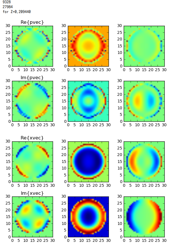
Fig2. From left to right: array[::3], array[1::3], arr[2::3].